
Online Mechanisms for Charging Electric Vehicles in Settings with Varying Marginal Electricity Costs
Proceedings of the Twenty-Fourth International Joint Conference on Artificial Intelligence. Special Track on Computational Sustainability. Pages 2610-2615.
© 2015 International Joint Conferences on Artificial Intelligence
Abstract
We propose new mechanisms that can be used by a demand response aggregator to flexibly shift the charging of electric vehicles (EVs) to times where cheap but intermittent renewable energy is in high supply. Here, it is important to consider the constraints and preferences of EV owners, while eliminating the scope for strategic behaviour. To achieve this, we propose, for the first time, a generic class of incentive mechanisms for settings with both varying marginal electricity costs and multidimensional preferences. We show these are dominant strategy incentive compatible, i.e., EV owners are incentivised to report their constraints and preferences truthfully. We also detail a specific instance of this class, show that it achieves ≈98% of the optimal in realistic scenarios and demonstrate how it can be adapted to trade off efficiency with profit.
- [Albadi and El-Saadany, 2007] M.H. Albadi and E.F. El- Saadany. Demand response in electricity markets: An overview. In Power Engineering Society General Meeting, 2007. IEEE, pages 1-5, June 2007.
- [Bhattacharya et al., 2014] S. Bhattacharya, K. Kar, J.H. Chow, and A. Gupta. Extended second price auctions for plug-in electric vehicle (pev) charging in smart distribu- tion grids. In American Control Conference (ACC), 2014, pages 908-913. IEEE, 2014.
- [Bikhchandani et al., 2006] S. Bikhchandani, S. Chatterji, R. Lavi, A. Mu'alem, N. Nisan, and A. Sen. Weak mono- tonicity characterizes deterministic dominant-strategy im- plementation. Econometrica, 74(4):1109-1132, 2006.
- [Bitar et al., 2011] E. Bitar, P.P. Khargonekar, and K. Poolla. Systems and control opportunities in the integration of re- newable energy into the smart grid. In Proc. of IFAC World Congress, pages 4927-4932, 2011.
- [Clement-Nyns et al., 2011] K. Clement-Nyns, E. Haesen, and J. Driesen. The impact of vehicle-to-grid on the distri- bution grid. Electric Power Systems Research, 81(1):185- 192, 2011.
- [Conejo et al., 2010] A.J. Conejo, J.M. Morales, and L. Baringo. Real-time demand response model. Smart Grid, IEEE Transactions on, 1(3):236-242, Dec 2010.
- [Gerding et al., 2011] E.H. Gerding, V. Robu, S. Stein, D.C. Parkes, A.C. Rogers, and N.R. Jennings. Online mech- anism design for electric vehicle charging. In The 10th International Conference on Autonomous Agents and Mul- tiagent Systems, pages 811-818, 2011.
- [Gkatzikis et al., 2013] L. Gkatzikis, I. Koutsopoulos, and T. Salonidis. The role of aggregators in smart grid de- mand response markets. Selected Areas in Communica- tions, IEEE Journal on, 31(7):1247-1257, July 2013.
- [Ipakchi and Albuyeh, 2009] A. Ipakchi and F. Albuyeh. Grid of the future. Power and Energy Magazine, IEEE, 7(2):52-62, 2009.
- [Mohsenian-Rad et al., 2010] A.-H. Mohsenian-Rad, V.W.S. Wong, J. Jatskevich, and R. Schober. Optimal and au- tonomous incentive-based energy consumption scheduling algorithm for smart grid. In Innovative Smart Grid Tech- nologies (ISGT), 2010, pages 1-6. IEEE, 2010.
- [Parkes, 2007] D.C. Parkes. Online mechanisms. In Nisan, N., Roughgarden, T., Tardos, E., and Vazirani, V. (Eds.) Algorithmic Game Theory, pages 411-439, 2007.
- [Robu et al., 2013] V. Robu, E.H. Gerding, S. Stein, D.C. Parkes, A.C. Rogers, and N.R. Jennings. An online mech- anism for multi-unit demand and its application to plug-in hybrid electric vehicle charging. Journal of Artificial In- telligence Research, 48:175-230, 2013.
- [Royal Academy of Engineering, 2010] Royal Academy of Engineering. Electric Vehicles: Charged with potential. Royal Academy of Engineering, 2010.
- [Saad et al., 2012] W. Saad, Z. Han, H.V. Poor, and T. Basar. Game-theoretic methods for the smart grid: An overview of microgrid systems, demand-side management, and smart grid communications. Signal Processing Magazine, IEEE, 29(5):86-105, 2012.
- [Stein et al., 2012] S. Stein, E.H. Gerding, V. Robu, and N.R. Jennings. A model-based online mechanism with pre- commitment and its application to electric vehicle charg- ing. In Proceedings of the 11th International Confer- ence on Autonomous Agents and Multiagent Systems (AA- MAS'12), pages 669-676, 2012.
- [Ströhle et al., 2014] P. Ströhle, E.H. Gerding, M. Weerdt, S. Stein, and V. Robu. Online mechanism design for scheduling non-preemptive jobs under uncertain supply and demand. In 13th International Conference on Au- tonomous Agents and Multi-Agent Systems, pages 437- 444, May 2014.
References were extracted automatically from the PDF and may contain errors.
Full text extracted automatically from the PDF; figures, tables and equations may differ. The PDF is the version of record.
1 Introduction
The widespread adoption of electric vehicles (EVs) is often seen as a vital step for mitigating climate change. Coupled with a shift towards clean renewable electricity generation, such as photovoltaics (PV) or wind energy, EVs promise to dramatically reduce emissions [Royal Academy of Engineering, 2010]. However, these renewable energy sources are typically intermittent and depend heavily on weather conditions [Bitar et al., 2011]. In particular, peaks in renewable energy supply (e.g., at noon for PV) may not coincide with peaks in demand (e.g., in the evening when EV owners plug in). Thus, more expensive and polluting conventional methods of electricity generation have to be used at those peak times.
To address this disparity in supply and demand, it is possible to exploit the flexibility of EV owners and delay charging to periods of higher renewable supply [Ipakchi and Albuyeh, 2009; Clement-Nyns et al., 2011]. In particular, recent work has suggested the introduction of demand response
Enrico H. Gerding
University of Southampton Southampton, United Kingdom eg@ecs.soton.ac.uk
Takahiro Shiga
Toyota Central R&D Labs., Inc. Aichi, Japan t-shiga@mosk.tytlabs.co.jp
services, whereby electricity consumers are offered financial incentives to shift their consumption [Albadi and ElSaadany, 2007]. Often, this is facilitated by an aggregator, which procures electricity from the wholesale electricity market and then coordinates the consumption of individual endusers [Gkatzikis et al., 2013]. This allows the aggregator to achieve significant cost savings.
As the end-consumers (i.e., EV owners) in these systems are self-interested agents, which balance the inconvenience of shifting their consumption with the associated financial incentives, there is considerable work on modelling this setting using game theory [Mohsenian-Rad et al., 2010; Saad et al., 2012; Bhattacharya et al., 2014]. Typically, coordination is achieved using real-time pricing mechanisms, which adjust electricity prices depending on demand and on the marginal costs of generation [Conejo et al., 2010]. However, participating in such a mechanism imposes a significant burden on EV owners, as they have to reason strategically about future demand in order to decide when to charge.
To address this, recent work has looked at coordinating the charging of EVs using online mechanism design [Parkes, 2007]. Specifically, Gerding et al. [2011] propose a scheduling and pricing mechanism that aggregates the multidimensional preferences of dynamically arriving EV owners and that ensures that truthful reporting of these preferences maximises each participant's utility (i.e., the mechanism is dominant strategy incentive compatible, or DSIC). This removes the need for strategic behaviour, allowing the mechanism to find a schedule with high efficiency. Other work uses the notion of pre-commitment to delay more flexible EV owners while retaining the DSIC property, albeit only for settings with single-dimensional preferences [Stein et al., 2012], and this is extended to deal with a demand response setting with variable renewable generation in [Str¨ohle et al., 2014].
However, these mechanisms do not consider the marginal cost of generation, which depends on the available supply of renewable energy and varies with the amount of energy that is consumed. Additionally, the mechanism in [Gerding et al.,
2011] is based on a simple greedy allocation and requires cancelling some allocations. This leads to very inefficient allocation decisions, especially when marginal costs are considered. To address these shortcomings, we make the following novel contributions:
- We characterise, for the first time, a general class of DSIC online mechanisms which deal with both marginal generation costs and multi-dimensional preferences.
- We describe one particular instance from this class of mechanisms which, in addition to being DSIC, is computationally efficient, scaling to hundreds of agents.
- We empirically benchmark this mechanism and show that it achieves near-optimal performance and significantly outperforms the current state of the art, which does not consider the marginal cost of generation.
2 Smart Charging SystemModel
We consider a smart EV charging system, which is implemented by a demand response aggregator. This aggregator acts as a broker between the EV owners and the electricity market. Specifically, it procures electricity for EV charging from a mixture of local renewable generators, possibly through long-term contracts, and the wholesale global electricity market. The aggregator also collects the constraints and preferences of individual EV owners and then schedules their charging to maximise social welfare and/or profit. This may involve shifting the charging of flexible EV owners to times where electricity is cheap or even curtailing consumption when prices are too high.
2.1 EVOwner Model
We consider a model with discrete and possibly infinite time steps t ∈ T. Each EV owner is represented by an agent, and we use I = {1, . . . , n} to denote the set of all agents. At every time step, an agent can charge a single unit of electricity (e.g., corresponding to 3 kWh), and we assume that all EVs charge at the same rate. Each agent i ∈ I has a limited availability for charging, which is given by an arrival time ai ∈ T (i.e., earliest possible time for charging) and a departure time di ∈ T (i.e., latest time for charging), with di ≥ ai. The agent's valuations for charging are given as a vector vi = {vi,1, vi,2, . . .}, where vi,k denotes the marginal value for the kth unit. We assume these are non-increasing, i.e., ∀k > j : vi,j ≥ vi,k, which is a natural assumption for plug-in hybrid EVs [Robu et al., 2013]. Given this, we use θi = {ai, di, vi} to summarise agent i's type. θ = {θ1, . . . , θn} denotes the types of all agents and θ-i denotes the types of all agents except i. Furthermore, we use I 〈t〉 and θ〈t〉 to denote the agents and their types in the market at or before time t.
From time ai, when agent i becomes available for charging (i.e., when the EV arrives at home and is plugged in), he can report his type to the aggregator, e.g., using a communication device that is integrated with his charging equipment or via a smart phone app. Crucially, we assume that the agent could strategically misreport his type, if this is in his best interest. Thus, we use ˆ θi = {ˆai, ˆ di, ˆ vi} to denote agent i's report (here, ˆai is given implicitly by the time the report is made). As is common in this domain, we assume that agents cannot report an earlier arrival or later departure time, i.e., ˆai ≥ ai and ˆ di ≤ di. This is a natural assumption in this domain, as a vehicle cannot be plugged into the charging equipment when it is unavailable for charging, but it is easy to delay plugging in, or to unplug early [Robu et al., 2013].
2.2 Aggregator Mechanism
Given the reported types of EV agents, the aggregator now uses a scheduling function πi,t(ˆ θ〈t〉 ), which keeps track of how many units of electricity have been allocated to agent i on or before time t. Importantly, as this is an online setting, this function can only depend on the types that have arrived on or before the current time t. Here, ∀t, ˆai ≤ t ≤ ˆ di : πi,t(ˆ θ〈t〉 ) - πi,t-1(ˆ θ〈t-1〉 ) ∈ {0, 1}, and this indicates whether agent i charges at time t.
When charging EVs, the aggregator also has to procure the necessary amount of electricity either from the global wholesale market or from local renewable sources. The cost for this depends both on the time of charging and on the amount of electricity that is needed. To model this, we use marginal costs c(t, m), which is the marginal cost for charging the mth vehicle at time t. Here, we assume that supply is infinite, i.e., any number of vehicles can be charged concurrently, but the associated marginal costs could be very high (reflecting, for example, the need to power up additional generators). Typically, c(t,m+ 1) ≥ c(t,m), but this is not a requirement for our mechanism. We also assume that costs are deterministic and known in advance, but they could reflect expected costs without changing the mechanisms presented here. Table 1 shows a part of the cost function used in the experiments.
In addition to deciding on a schedule, the mechanism also determines a payment xi(ˆ θ〈 ˆ di〉 ) for each agent i, which has to be paid on his departure. As before, this can only depend on the reported types up to the current time. This payment, along with the scheduling decisions, can be designed to ensure certain desirable properties in strategic settings, which we briefly discuss in the following section.
Given this, the aggregator's goal could be to maximise social welfare, denoted by SW(θ), which is the sum of marginal values minus the sum of marginal costs. Formally, let M π t denote the number of units allocated at time t, then:
SW ( ˆ θ) = ∑i∈I ∑πi, ˆ di ( ˆ θ) j=1 ˆ vi,j - ∑t∈T ∑Mπ t m=1 c(t,m). An alternative goal is to maximise profit, which is the total payments received minus the total costs: ∑i∈I xi(ˆ θ〈 ˆ di〉 ) - ∑t∈T ∑Mπ t m=1 c(t, m). We consider both goals in Section 4.
2.3 Strategic Behaviour
We assume that EV owners are self-interested, and so we model them as rational utility-maximisers. Specifically, the utility of an agent i with type θi and who reports ˆ θi (while all other agents report ˆ θ-i) is given by Ui({ˆ θ-i, ˆ θi}, θi) =
As a result, we must assume that agents will misreport their types if this increases their own utility. To address this, we aim to design a scheduling function πi,t and payment xi that ensure the mechanism is dominant strategy incentive compatible (DSIC), i.e., agents maximise their utility when reporting their own types truthfully. Formally, we want to ensure that ∀θi, ˆ θi, ˆ θ-i : Ui({ˆ θ-i, θi}, θi) ≥ Ui({ˆ θ-i, ˆ θi}, θi).
3 ProposedMechanism
In what follows we first introduce a generic mechanism and then show that it satisfies the DSIC property in our setting. The mechanism is generic, as it can be used with a variety of pricing rules and (possibly sub-optimal) scheduling algorithms. To achieve DSIC, it simply imposes certain constraints on these rules and algorithms. We then introduce a specific pricing rule and scheduling heuristic that satisfy these constraints and which are used in the experiments.
3.1 Generic Mechanism
Unlike standard mechanism design approaches, which define a (weakly) monotonic allocation and then use critical value payments to ensure DSIC [Bikhchandani et al., 2006], we take a different approach. First, for each agent i, a minimum price for charging at every time step t is determined, using a pricing function f. These prices, combined with an agent's valuation function and his availability in the market, determine the maximum number of units, li, which need to be allocated to the agent by his departure time. Importantly, prices can increase over time if more agents (with potentially higher valuations) enter the market later and so the allocation to agent i can decrease.
However, this has to be done carefully. Allocations have to remain feasible by an agent's departure time, agents with a longer availability cannot be penalised through these revised allocations, and, to avoid cancellations, the mechanism must never charge more units than an agent would like, given the final prices. To ensure these properties, we derive general conditions on prices and allocations. The full process, which is performed for each agent i, is detailed below.
Calculating theminimummarginal price vector We start by computing the minimum marginal payment vector at time t, pi 〈t〉 , where p〈t〉 i,j is the (minimum) payment for the j th unit of electricity. To this end, we first determine the prices of charging at specific times in the market. We distinguish between past units, for which the prices are fixed, and future units, for which the prices can still increase. Let f(ˆ θ〈t〉 -i , t′ ) denote a function which determines the price of a unit of electricity at any time t′ ≥ t in the future. For brevity we use f 〈t〉 i,t′ = f(ˆ θ〈t〉 -i , t′ ). We discuss a specific example function in Section 3.3, but the mechanism can support any function as long as it does not depend on θi and it satisfies:
That is, prices at specific times in the future t′ > t can only increase or remain unchanged as the actual time, t, approaches these time points. 1 A trivial example satisfying this constraint is where prices are always zero. However, in that case the aggregator will make a loss if costs are strictly positive.
Once we reach a certain time step, the prices at that time are fixed and no longer change. Formally, if t is the current time step, and the current price is given by f 〈t〉 i,t , then:
Given this, we can compute a price vector at time t as follows:
Note that this vector consists of two parts: the prices from the agent's reported arrival, ˆai, up to the current time, t, are fixed, whereas the remaining prices are future prices and so they can still increase.
Now, the price vector ηi 〈t〉 determines the prices at different time steps, but the agent is not interested in when it is allocated the units but would simply like the cheapest ones within the period that he is available in the market. To ensure that the agent always gets the best price (which is not necessarily the price at the time he is charged by the scheduling mechanism), we sort the prices in ascending order to obtain the minimum marginal payment vector:
where incr(.) is an operator which arranges the input vector in ascending order.
Determining the scheduling constraints We now compute the number of units to be assigned to agent i by his reported departure, ˆ di, given the current prices, pi 〈t〉 , and the agent's valuation vi, such that his utility is maximised. Specifically:
Note that ˆ di -ˆai +1 is an upper bound on the number of units which can be allocated within the time that the agent is available in the market. As a result, even if prices are zero, the mechanism never allocates more than is physically possible (recall that we assume unlimited supply). Henceforth we refer to li 〈t〉 as the temporarily assigned number of units, which is imposed on the scheduling algorithm (as detailed below).
The temporarily assigned number of units includes possible future allocations (up to the agent's reported deadline). Therefore, if prices increase, the number of assigned units could decrease over time. In order to prevent the mechanism from over-allocating units, which then later would need to be cancelled, we impose an additional constraint on the number of units which the scheduler can allocate up to the current time. This constraint uses only the fixed prices from the price vector. Specifically, let:
1 This is not a major restriction as typically new agents entering the market in the future will push up prices.
denote the vector of fixed prices. Similarly, p′i 〈t〉 = incr(η′i 〈t〉 ) and l′i 〈t〉 is given by:
Note that the upper bound of l′i is t-ˆai +1. We refer to l′i 〈t〉 as the upper limit allocation for agent i at time t.
Scheduling algorithm We now proceed with the actual allocation of units to agents. As with the prices, we consider both the past allocations as well as future allocations. Let π〈t〉 i,t′ = πi(θ〈t〉 , t′ ) denote a scheduling algorithm which specifies the total number of units allocated to agent i by time t′ when the current time is t. Note that, since we have that only a single unit can be allocated per time step, necessarily ∀t′ , t : π〈t〉 i,t′+1 - π〈t〉 i,t′ ≤ 1. Note that this is an extension of the notation introduced in Section 2.2, which allows the scheduling algorithm to make (potentially temporary) allocation decisions for future time t′ > t, given the information available at time t. Specifically, π〈t〉 i,t = πi,t. Naturally, the scheduling algorithm cannot change past allocations and so:
In terms of future allocations, any allocation function can be used, as long as it meets the following constraints at every t:
That is, by the reported deadline agent i needs to be able to receive its temporarily assigned number of units. Note that this future allocation can still decrease over time (when prices increase), but it should be possible to allocate the necessary number of units if prices and corresponding allocations do not change. At the same time, it needs to meet the constraint:
That is, the scheduler cannot assign more than the upper limit allocation by the current time. In Section 3.2 we show that, provided that the pricing conditions are met, these constraints can always be satisfied.
Payment Finally, the payment, which is computed on the (reported) departure of agent i, is given by:
3.2 Theoretical Properties
Before we show that the proposed class of mechanisms is always DSIC, we first show that Eqs. 8 and 9 can always be satisfied using a feasible schedule.
Definition 1 (Feasible schedule). A schedule is feasible if ∀t : π〈t〉 i,t - π〈t-1〉 i,t-1 ∈ {0, 1}, i.e., we assign at most one unit per time step, and we do not reduce the allocations.
Lemma 1. Given unlimited supply and given that ˆvi, i ∈ I are marginally non-increasing, if Eqs. 8 and 9 are satisfied at time t - 1, there always exists a feasible schedule which satisfies the equations at time t.
Proof. First we show π〈t〉 i,t - π〈t-1〉 i,t-1 ≥ 0, i.e., the constraints never lead to a decrease in actual allocations. Because a new price is added to the fixed price vector at each time step, we have that l′i 〈t〉 ≥ l′i 〈t-1〉 , i.e., the upper limit allocation can only increase. At the same time, because future prices increase, we have that li 〈t〉 ≤ li 〈t-1〉 , i.e., the temporarily assigned number of units can decrease. However, this can never go below the upper limit allocations. In particular: li 〈t〉 ≥ l′i 〈t-1〉 . To see this, note that all fixed prices in p′i 〈t-1〉 are also in pi 〈t〉 . Therefore, with more (possibly lower) prices to choose from, the allocation which maximises the agent's utility, Eq. 5, is at least as high Eq. 6.
To ensure that π〈t〉 i,t -π〈t-1〉
i,t-1 ≤ 1, we consider two cases. Case 1: π〈t-1〉 i,t-1 < l′i 〈t′ 〉 . In this case, given that the constraints are satisfied at t - 1, because li 〈t〉 ≤ li 〈t-1〉 we can always satisfy both constraints at time t by charging at time t, i.e., by setting π〈t〉 i,t = π〈t-1〉 i,t-1 +1.
Case 2: π〈t-1〉 i,t-1 = l′i 〈t′ 〉 . In this case, in order to satisfy Eq. 9 we cannot charge at time t. We have to show that we can still satisfy Eq. 8. Note that such a schedule is feasible as long as li 〈t〉 - l′i 〈t〉 ≤ ˆ di - t, i.e., the total number of units to be allocated by the deadline is at most the number of remaining time steps (since we can only allocate at most one unit per time step). Note that pi 〈t〉 contains all the prices in p′i 〈t〉 plus exactly ˆ di - t additional values. In addition, the differences in the upper bounds is also exactly ˆ di - t (in particular, note that p′i 〈 ˆ di〉 = pi 〈 ˆ di〉 . Therefore, provided that the marginal valuations are non-increasing, we have that the difference between li 〈t〉 and l′i 〈t〉 is at most ˆ di - t. 2
Lemma 2. There always exists a feasible schedule where Constraints 8 and 9 can be satisfied on arrival.
The above results not only imply that a feasible schedule always exists but, more importantly, any existing scheduling algorithm can be adapted by simply introducing the necessary constraints at each time step, which automatically ensures that the constraints can be satisfied in the next time step. We now show that the constraints always lead to the mechanism being DSIC.
Theorem 1. Given limited misreports and non-increasing marginal valuations ˆ vi of agents i ∈ I, any mechanism with pricing function f(ˆ θ〈t〉 -i , t′ ) satisfying Eq. 1 and scheduling algorithm satisfying Eq. 8 is DSIC.
2 The assumption that marginal valuations are non-increasing is important here. Suppose otherwise, e.g., vi = {0, 0, 10}, ˆai = 1, ˆ di = 3, p′i 〈2〉 = {1, 1} and pi 〈2〉 = {1, 1, 1}, we have that l′i 〈2〉 = 0 and li 〈2〉 = 3, resulting in an infeasible schedule since π〈2〉 i,3 -π〈2〉 i,2 = 3 - 0 = 3.
Proof. (1) We show that, regardless of the reported arrival and departure, it is a dominant strategy to truthfully report vi. (2) We then show that, given vi = ˆvi, there is no incentive to report a later arrival or an earlier departure.
(1) Given that pricing function f does not depend on θi, the marginal prices on departure of agent i, pi 〈 ˆ di〉 , only depend on ˆai and ˆ di, and not on ˆvi. Therefore the agent cannot influence the prices by misreporting vi but only the allocation. For a given allocation πi, and payments according to Eq. 10, the utility of agent i is given by: ∑πi j=1 (vi,j - p〈 ˆ di〉 i,j ). Due to Constraint 8, the allocation on (reported) departure maximises Eq. 5, which corresponds to the agent's utility when vi = ˆvi. Therefore, reporting vi truthfully is optimal.
(2) Suppose that the agent reports a later arrival, ˆai > ai. According to Eq. 1 we have that f 〈ˆai〉 i,t ≥ f 〈ai〉 i,t , which means that prices for the same corresponding time period in price vector η〈 ˆ di〉 i can increase (and never decrease). In addition, η〈 ˆ di〉 i contains ˆai - ai fewer prices. Because the marginal payment vector pi 〈 ˆ di〉 is in ascending order, the payment can only increase by having fewer prices. Now suppose that ˆ di < di. Let η〈 ˆ di〉 i = {f 〈ˆai〉 i,ˆai , . . . , f 〈 ˆ di〉 i, ˆ di } denote the final price vector when misreporting, and let η〈di〉 i = {f 〈ˆai〉 i,ˆai , . . . , f 〈 ˆ di〉 i, ˆ di , f 〈 ˆ di+1〉 i, ˆ di+1 , . . . , f 〈di〉 i,di } denote the final prices using the agent's true departure. Note that, in both cases, the first ˆ di - ˆai + 1 prices are identical. Therefore, by misreporting an earlier departure, the price vector only contains fewer prices. This means marginal payments can only increase.
3.3 Specific Mechanism
Although our approach guarantees DSIC for a range of pricing functions and scheduling algorithms, a poor choice can lead to poor efficiency and a loss for the aggregator if it cannot recoup the incurred marginal costs from the suppliers (formally, our class of mechanisms does not guarantee weak budget balance). In this section we demonstrate our approach for a specific pricing function and scheduling algorithm, which we then evaluate empirically in Section 4.
Pricing Function In this section we instantiate the pricing function f(ˆ θ〈t〉 -i , t′ ). Note that different prices need to be calculated for each agent i ∈ I, and we cannot use agent i's type when doing so. In addition we need to calculate prices for each future time point t′ , where t ≤ t′ ≤ ˆ di. To reduce the computational costs, we use a heuristic approach.
In detail, we run a virtual version of the market without agent i and with all known agents ˆ θ〈t〉 -i , and we allocate the units to those agents in a greedy manner as follows. 3 We take the agent with the highest marginal value, and allocate this agent the unit with the lowest available marginal cost given the agent's arrival and departure time, and provided that the marginal value is equal to or higher than the marginal cost (otherwise no match is made). We remove the matched values and costs from the market, and we repeat this process until no more matches can be made. Let SW(ˆ θ〈t〉 -i ) denote the social welfare of the resulting allocation.
3 The market needs to be run from before the first arrival, e.g., when the market first started or from the beginning of each day (denoted by t1).
Now, to compute the prices at time t′ , we allocate a single unit at time t′ to agent i and we rerun the market as before. Let SWt′ (ˆ θ〈t〉 -i ) denote the social welfare of the resulting allocation, excluding agent i's value for the unit. Given this, the pricing function for agent i is defined as follows.
Intuitively, the payment is the externality imposed on the system excluding agent i if a unit at time t′ is allocated to i. 4 Note that the max operator ensures that Eq. 1 always holds.
Scheduling Algorithm To determine the prices we used a fast heuristic scheduling algorithm since this needs to be repeated for each agent and future time step. Also, for the prices we did not need to consider the scheduling constraints. In contrast, the scheduling algorithm for the actual allocation needs to be computed only once at every current time step. Hence, for the allocation we optimise the social welfare considering all agents, subject to Eqs. 8 and 9 for each agent. The optimization is executed by solving a Mixed Integer Program (MIP) using the Gurobi 5 solver with a tolerance of 10-4 . Note that, although this algorithm is near-optimal, this is not a requirement for the mechanism to satisfy DSIC.
4 Numerical Analysis
To quantify the performance of our proposed mechanism in realistic demand response settings, we now evaluate it numerically, comparing it to existing state-of-the-art mechanisms.
4.1 Experimental Setup
We determine the hourly marginal costs c(t,m) of a 24-hour period of a typical day as follows. For electricity prices we use the data from the Japan Electric Power Exchange 6 on the 5th of June, 2013. To determine the costs, in addition we use the typical energy consumption of Japanese households on a fine June day 7 . Taking regular household consumption into account is important, since EV charging will use energy on top of what is normally consumed. Furthermore, we assume that the charging rate of all agents is 3kW, and so a single unit is 3kWh. Details are omitted due to space constraints but a small sample is shown in Table 1. Here, c(13, 1) = 0.1 is the cost in JPY for charging a single vehicle at time step 13. The marginal cost for the second vehicle is c(13, 2) = 8.2, resulting in a total cost of 8.3 JPY for charging both.
4 The intuition is similar to the well-known Vickrey-ClarkeGroves mechanism for static settings, but our approach does not assume optimality and only considers a single unit at a time.
5 http://www.gurobi.com/
6 http://www.jepx.org/english/index.html
7 We use data from the Architectural Institute of Japan, see http://tkkankyo.eng.niigata-u.ac.jp/HP/HP /database/index.htm.
| time(t) | |||||
|---|---|---|---|---|---|
| 13 | 14 | 15 | 16 | ||
| number of agents (m) | 1 | 0.1 | 0.1 | 42.7 | 66.1 |
| 2 | 8.2 | 0.2 | 60.1 | 66.2 | |
| 3 · · | 57.9 | 0.3 | 60.9 · | 66.3 | |
To obtain the distribution of the agents' arrival and departure times, we use the results from a questionnaire of 340 citizens in Nagoya City in Japan, which asked about daily movements. From this questionnaire we use the answers regarding when and for how long cars were parked at home during weekdays. For the simulations, each agent's arrival-departure pair is randomly selected from the 340 samples. Finally, the remaining capacity of each agent is randomly chosen between 1 and 6 units of charge. For each unit, the agent's marginal valuation is uniformly drawn from 0 to 100 JPY and these are arranged in descending order.
4.2 BenchmarkMechanisms
We compare the performance of the mechanism from Section 3.3, called Proposed, with those from the literature.
Greedy optimally allocates the available electricity in each time step without considering future time steps. As noted in [Gerding et al., 2011], this mechanism violates weak monotonicity and therefore is not truthful in settings with multidimensional valuations (even when costs are zero).
Greedy with cancellation on departure (GCOD) works like Greedy except that allocations are sometimes cancelled on departure as specified in [Gerding et al., 2011] to ensure DSIC.
First Come First Serve (FCFS) optimally schedules each agent in order of their arrival. If multiple agents arrive at the same time, they are scheduled in order of their ID, which is assigned to all agents beforehand. This mechanism is DSIC when the payment is set equal to the incurred marginal costs (but the aggregator makes no profit).
Myopically Optimal (MO) optimises social welfare using all information currently available. The allocations are recalculated whenever a new agent enters the market. This is the same scheduling mechanism used in Section 3.3 without considering the constraints, and is not DSIC.
Optimal uses the same algorithm as MO but assumes perfect foresight of the agents arriving in the future.
4.3 Results
We first compare the efficiency, which is the obtained social welfare as a proportion of the Optimal. To this end, we vary the number of agents from 10 to 300, and for each setting we run 1000 trials. Each trial simulates a 48-hour period, and the cost table is assumed to be the same for these two days.
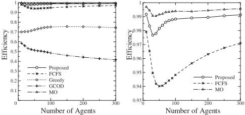
The results in Figure 1 show that Proposed is very close to Optimal. As expected, MO outperforms Proposed since the former is not bound by the constraints. However, Proposed outperforms all other DSIC mechanisms, especially GCOD and even Greedy. GCOD performs especially poorly due to the costs which are still incurred even if the allocation is cancelled (and so the electricity is unused). Note that the efficiency of the top three mechanisms first decreases when the number of agents is less than 30 agents, and then increases. This is because, when there are few agents, scheduling is relatively easy since there is little competition. When there are a lot of agents, many of them will have similar high marginal values and so it does not matter too much which of them are scheduled. The fact that this happens around 30 is mainly due to the cost table used.
Surprisingly, the simple mechanism FCFS also performs very well in terms of efficiency, whilst also being DSIC. However, as mentioned in Section 4.2, no profit is made by the aggregator since the payment is equal to the marginal costs.
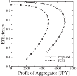
A simple way for the aggregator to increase profits of any mechanism (whilst maintaining DSIC) is to artificially increase costs by a constant, and pocket the difference. However, as with reserve prices, this lowers efficiency. In this part, we compare the mechanisms Proposed and FCFS in terms of their trade off between profit and efficiency. Specifically, we multiply the costs used in the pricing rule by a constant, α.
To this end, Figure 2 shows the relation between efficiency and aggregator profit for different values of α, where α is varied from 1.0 to 2.5. The number of agents is set to 200, and each point shows the average over 1000 trials. Here, efficiency is w.r.t. the Optimal with original costs. The top left is where α = 1. As we increase α, as expected, initially the profit increases for both mechanisms, but eventually the profit decreases (since the efficiency becomes very low). Comparing the two mechanisms, we can see that the Proposed mechanism is able to obtain ≈ 44% higher profits than FCFS whilst having the same efficiency. Conversely, for the same level of profit, the efficiency of Proposed is considerably higher.
Finally, we briefly comment on the computational tractability. Even though Proposed requires more computation than the other approaches, it is scalable to hundreds of agents. For example, a 48-hour trial with 300 agents takes 52 seconds on average on an Intel(R)Core(TM)i7-4770K CPU @ 3.50GHz using a single core.
5 Conclusions
We have proposed a novel approach for designing online mechanisms for multi-dimensional valuations and marginal costs. The approach can be used in combination with any pricing and allocation function, subject to a set of constraints being met. We have shown that the constraints are always feasible in settings with marginally non-increasing valuations and that the resulting mechanisms are DSIC. We have empirically compared an instantiation and have shown that, in a realistic setting with varying marginal costs, our mechanism outperforms existing DSIC mechanisms in terms of efficiency and profit. It is also computationally efficient and scales to hundreds of agents.
In future, we plan to extend the mechanisms to allow for multiple units to be allocated to an agent in a single time step (to capture settings where EVs can be charged at different rates). Moreover, we will consider mechanisms for settings where the marginal valuations of agents can be increasing.
@inproceedings{ijcai2015p370,
  title     = {Online Mechanisms for Charging Electric Vehicles in Settings with Varying Marginal Electricity Costs},
  author    = {Hayakawa, Keiichiro and Gerding, Enrico H. and Stein, Sebastian and Shiga, Takahiro},
  booktitle = {Proceedings of the Twenty-Fourth International Joint Conference on
               Artificial Intelligence, {IJCAI-15}},
  publisher = {International Joint Conferences on Artificial Intelligence},
  editor    = {Qiang Yang and Michael Wooldridge},
  pages     = {2610--2615},
  year      = {2015},
  month     = {7},
  note      = {Special Track on Computational Sustainability},
  url       = {https://ijcai.org/proceedings/2015/370},
}
TY - CPAPER TI - Online Mechanisms for Charging Electric Vehicles in Settings with Varying Marginal Electricity Costs AU - Hayakawa, Keiichiro AU - Gerding, Enrico H. AU - Stein, Sebastian AU - Shiga, Takahiro T2 - Proceedings of the Twenty-Fourth International Joint Conference on Artificial Intelligence, IJCAI-15 PB - International Joint Conferences on Artificial Intelligence PY - 2015 SP - 2610 EP - 2615 UR - https://ijcai.org/proceedings/2015/370 ER -Copied
Machine-readable versions of this paper, for tools and AI agents:





