
Exploiting Symmetries by Planning for a Descriptive Quotient
Proceedings of the Twenty-Fourth International Joint Conference on Artificial Intelligence. Main Track. Pages 1479-1485.
© 2015 International Joint Conferences on Artificial Intelligence
Abstract
We eliminate symmetry from a problem before searching for a plan. The planning problem with symmetries is decomposed into a set of isomorphic subproblems. One plan is computed for a small planning problem posed by a descriptive quotient, a description of any such subproblem. A concrete plan is synthesized by concatenating instantiations of that one plan for each subproblem. Our approach is sound.
- [Amir and Engelhardt, 2003] Eyal Amir and Barbara Engel- hardt. Factored planning. In IJCAI, volume 3, pages 929- 935. Citeseer, 2003.
- [Brafman and Domshlak, 2006] Ronen I Brafman and Carmel Domshlak. Factored planning: How, when, and when not. In AAAI, volume 6, pages 809-814, 2006.
- [Brown et al., 1996] Cynthia A. Brown, Larry Finkelstein, and Paul Walton Purdom Jr. Backtrack searching in the presence of symmetry. Nord. J. Comput., 3(3):203-219, 1996.
- [Clarke et al., 1998] Edmund M Clarke, E Allen Emerson, Somesh Jha, and A Prasad Sistla. Symmetry reductions in model checking. In Computer Aided Verification, pages 147-158. Springer, 1998.
- [Crawford et al., 1996] James Crawford, Matthew Ginsberg, Eugene Luks, and Amitabha Roy. Symmetry-breaking predicates for search problems. KR, 96:148-159, 1996.
- [de Moura and Bjørner, 2008] Leonardo de Moura and Nikolaj Bjørner. Z3: An efficient SMT solver, 2008.
- [Domshlak et al., 2012] Carmel Domshlak, Michael Katz, and Alexander Shleyfman. Enhanced symmetry break- ing in cost-optimal planning as forward search. In ICAPS, 2012.
- [Domshlak et al., 2013] Carmel Domshlak, Michael Katz, and Alexander Shleyfman. Symmetry breaking: Satisfic- ing planning and landmark heuristics. In ICAPS, 2013.
- [Eugene, 1993] M Eugene. Permutation groups and polynomial-time computation. In Groups and Computa- tion: Workshop on Groups and Computation, October 7- 10, 1991, volume 11, page 139. American Mathematical Soc., 1993.
- [Fox and Long, 1999] Maria Fox and Derek Long. The de- tection and exploitation of symmetry in planning prob- lems. In Proceedings of the Sixteenth International Joint Conference on Artificial Intelligence, IJCAI 99, Stock- holm, Sweden, July 31 -August 6, 1999. 2 Volumes, 1450 pages, pages 956-961, 1999. IJCAI
- [Fox and Long, 2002] Maria Fox and Derek Long. Extend- ing the exploitation of symmetries in planning. In Pro- ceedings of the Sixth International Conference on Arti- ficial Intelligence Planning Systems, April 23-27, 2002, Toulouse, France, pages 83-91, 2002.
- [Guere and Alami, 2001] Emmanuel Guere and Rachid Alami. One action is enough to plan. In Proceedings of the Seventeenth International Joint Conference on Artificial Intelligence, IJCAI 2001, Seattle, Washington, USA, August 4-10, 2001, pages 439-444, 2001.
- [Helmert et al., 2014] Malte Helmert, Patrik Haslum, Jörg Hoffmann, and Raz Nissim. Merge-and-shrink abstrac- tion: A method for generating lower bounds in factored state spaces. Journal of the ACM (JACM), 61(3):16, 2014.
- [Joslin and Roy, 1997] David Joslin and Amitabha Roy. Ex- ploiting symmetry in lifted CSPs. In Proceedings of the Fourteenth National Conference on Artificial Intelligence and Ninth Innovative Applications of Artificial Intelligence Conference, AAAI 97, IAAI 97, July 27-31, 1997, Provi- dence, Rhode Island., pages 197-202, 1997.
- [Kelareva et al., 2007] Elena Kelareva, Olivier Buffet, Jinbo Huang, and Sylvie Thiébaux. Factored planning using de- composition trees. In IJCAI, pages 1942-1947, 2007. IJCAI
- [McKay and Piperno, 2014] Brendan D. McKay and Adolfo Piperno. Practical graph isomorphism, {II}. Journal of Symbolic Computation, 60(0):94 -112, 2014.
- [Miguel, 2001] Ian Miguel. Symmetry-breaking in planning: Schematic constraints. In Proceedings of the CP01 Work- shop on Symmetry in Constraints, pages 17-24, 2001.
- [Pochter et al., 2011] Nir Pochter, Aviv Zohar, and Jeffrey S Rosenschein. Exploiting problem symmetries in state- based planners. In AAAI, 2011.
- [Porco et al., 2013] Aldo Porco, Alejandro Machado, and Blai Bonet. Automatic reductions from PH into STRIPS or how to generate short problems with very long solutions. In ICAPS, 2013.
- [Richter and Westphal, 2010] Silvia Richter and Matthias Westphal. The LAMA planner: Guiding cost-based any- time planning with landmarks. Journal of Artificial Intel- ligence Research, 39(1):127-177, 2010.
- [Rintanen and Gretton, 2013] Jussi Rintanen and Charles Gretton. Computing upper bounds on lengths of transition sequences. In IJCAI, 2013. IJCAI
- [Rintanen, 2003] Jussi Rintanen. Symmetry reduction for SAT representations of transition systems. In ICAPS, pages 32-41, 2003.
- [Shleyfman et al., 2015] Alexander Shleyfman, Michael Katz, Malte Helmert, Silvan Sievers, and Martin Wehrle. Heuristics and symmetries in classical planning. In AAAI, 2015.
- [Sievers et al., 2015] Silvan Sievers, Martin Wehrle, Malte Helmert, Alexander Shleyfman, and Michael Katz. Fac- tored symmetries for merge-and-shrink abstractions. In Proc. 29th National Conf. on Artificial Intelligence. AAAI Press, 2015.
- [Wahl and Donaldson, 2010] Thomas Wahl and Alastair F. Donaldson. Replication and abstraction: Symmetry in automated formal verification. Symmetry, 2(2):799-847, 2010.
References were extracted automatically from the PDF and may contain errors.
Full text extracted automatically from the PDF; figures, tables and equations may differ. The PDF is the version of record.
1 Introduction
The planning and model checking communities have for some time sought methods to exploit symmetries that occur in transition systems. The quintessential planning scenario which exhibits symmetries is GRIPPER. This comprises a robot whose left and right grippers can be used interchangeably in the task of moving a set of N indistinguishable packages from a source location to a goal location. Intuitively the left and right grippers are symmetric because if we changed their names, by interchanging the terms left and right in the problem description, we are left with an identical problem. Packages are also interchangeable and symmetric.
One method to exploit symmetry is to perform checking of properties of interest-e.g., goal reachability-in a quotient system, which corresponds to a (sometimes exponentially) smaller bisimulation of the system at hand. Wahl and Donaldson (2010) review the related model checking literature. Such methods were recently adapted for planning and studied by Pochter et al. (2011), Domshlak et al. (2012; 2013) and Shleyfman et al. (2015). Related work about statebased planning in equivalence classes of symmetric states includes [Guere and Alami, 2001; Fox and Long, 1999; 2002].
Planning in a quotient system, a state s is represented by a canonical element from its orbit, the set of states which are symmetric to s. Giving integer labels to packages in GRIPPER, when the search encounters a state where the robot is holding 1 package using 1 gripper, this is represented using the canonical state where, for example, the left gripper is holding package with identity "1". Orbit search explores the quotient system by simulating actions from known canonical states, and then computing the canonical representations of resultant states. That canonicalisation step requires the solution to the constructive orbit problem [Clarke et al., 1998] which is NP-hard [Eugene, 1993]. A key weakness, is that for each state encountered by the search an intractable canonicalisation operation is performed. This is mitigated in practice by using approximate canonicalisation. By forgoing exact canonicalisation, one encounters a much larger search problem than necessary. For a GRIPPER instance with 42 packages, the breadth-first orbit search with approximate canonicalisation by Pochter et al. reportedly performs 60.5K state expansion operations, far more than necessary.
∗NICTA is funded by the Australian Government through the Department of Communications and the Australian Research Council through the ICT Centre of Excellence Program.
Following the seminal work by Crawford et al. (1996) and Brown et al. (1996), when planning via constraint satisfaction, known symmetries are exploited by: (i) including symmetry breaking constraints, either directly as part of the problem expression [Joslin and Roy, 1997; Rintanen, 2003], or (ii) otherwise dynamically as suggested by [Miguel, 2001] as part of a nogood mechanism. In GRIPPER, we can statically require that if no package is yet retrieved, then any retrieval targets package 1 with the left gripper. Dynamically, having proved that no 3-step plan exists retrieving package 1 with the left gripper, then no plan of that length exists retrieving package i ̸= 1 using either gripper. Searching using the proposed dynamic approach is quite weak, as symmetries are only broken as nogood information becomes available. A weakness of both approaches is that problems expressed as CSPs include variables describing the state of the transition system at different plan steps. Existing approaches do not break symmetries across steps, and can therefore waste effort exploring partial assignments that express executions which visit symmetric states at different steps.
Our contribution is a novel procedure for domainindependent planning with symmetries. Following, e.g., Pochter et al., in a first step we infer knowledge about problem symmetries from the description of the problem. Then departing from existing approaches, our second step uses that knowledge to obtain a quotient of the concrete problem description. Called the descriptive quotient, this describes any element in the set of isomorphic subproblems which abstractly model the concrete problem. Third, we invoke a planner once to solve the small problem posed by that descriptive quotient. In the fourth and final step, a concrete plan is synthesized by concatenating instantiations of that plan for each isomorphic subproblem. The descriptive quotient of the aforementioned 42-package GRIPPER instance is solved by breadth-first search expanding 6 states. Using our approach, a concrete plan is obtained in under a second. For comparison, LAMA [Richter and Westphal, 2010] takes about 28 seconds.
The non-existence of a plan for the descriptive quotient does not exclude the possibility of a plan for the concrete problem. Although sound, in that respect our approach is incomplete. Having an optimal plan for the quotient does not guarantee optimality in the concatenated plan. Aside from computing a plan for the descriptive quotient, the computationally challenging steps occur in preprocessing:
- (i) Identification of problem symmetries from the original description, a problem as hard as graph isomorphism, which is not known to be tractable, and
- (ii) Computing an appropriate set of sub-problems isomorphic to the quotient.
2 Definitions and Notations
We formally define planning problems and related concepts. Where we do not refer to a specific function, we shall use the symbol f. We formalise functions as sets of key-value pairs (k ↦→ v). We use the term domain mathematically. We write D(f) for the domain of f, i.e., {k | (k ↦→ v) ∈ f}. We write R(f) for the range of f, i.e., {v | (k ↦→ v) ∈ f}.
Definition 1 (States and Actions). A planning problem is defined in terms of states and actions:
- (i) States are finite maps from variables-i.e., statecharacterizing propositions-to Booleans.
- (ii) An action a is a pair of finite maps over subsets of those variables. The first component of the pair, written pre(a), is the precondition and the second component of the pair (eff(a)) is the effect. The domain of an action is the union of the domains of the two finite maps. For a set of actions A, we define the set of preconditions pre(A) as ⋃a∈A pre(a).
We give examples of states and actions using sets of literals. For example, {x, y, z} is the state where state variables x and z are (map to) true, and y is false.
Definition 2 (Planning Problem). A planning problem Π is a 3-tuple 〈I, A, G〉, with I the initial state of the problem, G a description of goal states (another finite map from variables to Booleans), and A a set of actions. We define the domain of the problem (D(Π)) to be domain of the initial state (D(I)). Problem Π is valid if D(G) ⊆ D(I), and all actions refer exclusively to variables that occur in D(I). We only consider valid problems. Hereafter we refer to the initial state, actions or goal of problem Π as Π.I, Π.A or Π.G respectively. We may also omit the Π if it is clear from the context, e.g. I for Π.I and Ai for Πi.A. A state s is valid with respect to a planning problem Π if D(s) = D(I).
Definition 3 (Action Execution and Plan). When an action a is executed at state s, written e(s, a), it produces a successor state s′ . If pre(a) ̸⊆ s, then s′ = s. Otherwise s′ is a valid state where eff(a) ⊆ s′ and s(x) = s′ (x) ∀x ∈ D(I) \ D(eff(a)). We lift e to sequences of executions, taking an action sequence ˙π as the second argument. So e(s, ˙π) denotes the state resulting from successively applying each action from ˙π in turn, starting from s. An action sequence is a plan/solution if its execution from I yields a goal state.
Definition 4 (Subproblem). Problem Π1 is a subproblem of Π2, written Π1 ⊆ Π2, if D(I1) ⊆ D(I2), and if A1 ⊆ A2.
Definition 4 purposefully does not consider problem goals. We later consider subproblems with a variety of goals which do not all correspond to concrete problem goals. We form a concrete plan by concatenating plans for subproblems with such varieties of goals. For example, we will consider subproblems from GRIPPER with only one package and one gripper, where the goal is to: (i) relocate that package according to the concrete goal, (ii) additionally free the gripper, and (iii) additionally have the robot relocate to its starting position. In this case a concrete plan is formed by concatenating plans for subproblems given for each distinct package.
We require a few additional notations. Let m be a finite map, e.g., a state s, the assignments pre(a), etc. Then, let fLmM be the image of m under function f: the map {f(k) ↦→ v | (k ↦→ v) ∈ m}. This is well-defined if f(k1) = f(k2) implies that m(k1) = m(k2). We lift this notion of image to other composite types. For example, we write fLΠM for the image of Π under f, where all finite maps in Π are transformed by f .
3 Computing Problem Symmetries
To exploit problem symmetries we must first discover them. We follow the discovery approach from [Pochter et al., 2011], restricting ourselves to Boolean-valued variables in D(Π). We assume familiarity with groups, subgroups, group actions, and graph automorphism groups. Symmetries in a problem description are defined by an automorphism group.
Definition 5 (Problem Automorphism Group). The automorphism group of Π is: Aut(Π) = {σ | σLΠM = Π}. Members of Aut (Π) are permutations on D(Π).
A graphical representation of Π is constructed so vertex symmetries in it correspond to variable symmetries in Π. We follow the graphical representation introduced in [Pochter et al., 2011].
Definition 6 (Problem Description Graph (PDG)). The (undirected) graph Γ(Π) for a planning problem Π, is defined as follows:
- (i) Γ(Π) has two vertices, v⊤ and v⊥, for every variable v ∈ D(Π); two vertices, ap and ae, for every action a ∈ A; and vertex vI for I and vG for G.
- (ii) Γ(Π) has an edge between v⊤ and v⊥ for all v ∈ D(Π); between ap and ae for all a ∈ A; between ap and v∗ if (v ↦→ ∗) ∈ pre(a), and between ae and v∗ if (v ↦→ ∗) ∈ eff(a); between v∗ and vI if (v ↦→ ∗) occurs in I; and between v∗ and vG if (v ↦→ ∗) occurs in G.
We write V (Γ) for the set of vertices, and E(Γ) for edges of a graph Γ.
The automorphism group of the PDG, Aut(Γ(Π)), is identified by solving an undirected graph isomorphism problem. The action of a subgroup of Aut(Γ(Π)) on V (Γ(Π)) induces a partition, called the orbits, of V (Γ(Π)). We can now define our quotient structures based on partitions P of D(Π).
Definition 7 (Quotient Problems and Graphs). Given partition P of D(Π), let Q map members of D(Π) to their equivalence class in P. The descriptive quotient is Π/P = QLΠM, the image of Π under Q. This is well-defined if P is a set of orbits. We assume that quotient problems are well-defined.
For graph Γ and a partition P of its vertices, the quotient Γ/P is the graph with a vertex for each p ∈ P. Γ/P has an edge between any p1, p2 ∈ P iff Γ has an edge between any v ∈ p1 and u ∈ p2.
To ensure correspondence between PDG symmetries and problem symmetries, we must ensure incompatible descriptive elements do not coalesce in the same orbit. For example, we cannot have action precondition symbols and statevariables in the same orbit.
Definition 8 (Well-formed Partitions). A partition of V (Γ(Π)) is well-formed iff:
- (i) Positive (v⊤) and negative (v⊥) variable assignment vertices only coalesce with ones of the same parity;
- (ii) Precondition (ap) and effect (ae) vertices only coalesce with preconditions and effects respectively, and
- (iii) Both vI and vG are always in a singleton.
A well-formed partition ˆ P defines a corresponding partition P of D(Π), so that Γ(Π)/ ˆ P is isomorphic to Γ(Π/P).
To ensure well-formedness, vertex symmetry is calculated using the coloured graph-isomorphism procedure (CGIP). Vertices of distinct colour cannot coalesce in the same orbit. Vertices of Γ(Π) are coloured to ensure the orbits correspond to a well-formed partition.
4 Computing the Set of Instantiations
Recapping, symmetries in Π are the basis of a partition P of its domain D(Π) into orbits. That exposes the descriptive quotient, Π/P, an abstract problem whose variables correspond to orbits of concrete symbols. Our task now is to compute a set of instantiations of the quotient which cover all the goal variables D(G). Called a covering set of isomorphic subproblems, by instantiating a quotient plan for each subproblem and concatenating the results we intend to arrive at a concrete plan. We describe a pragmatic approach to obtaining that covering set. We establish that a covering set is not guaranteed to exists, and give an approach to refining partitions to mitigate that fact. We derive a theoretical bound on the necessary size of a covering set, and prove that a general graph formulation of the problem of computing a covering instantiation is NP-complete.
Definition 9 (Transversals, Instantiations). A transversal ⋔ is an injective choice function over P such that ⋔(c) ∈ c for every equivalence class c ∈ P. A transversal covers v if v ∈ R(⋔). If P is a partition of D(Π), we refer to a transversal ⋔ of P as an instantiation of Π/P. An instantiation ⋔ is consistent with a concrete problem Π if ⋔LΠ/PM ⊆ Π. When we use the term "problem" discussing an instantiation ⋔, we intend ⋔LΠ/PM. Note that D(⋔LΠ/PM) = R(⋔).
Example 1. Consider the set {a, b, c, d, e, f}, and the equivalence classes c1 = {a, b}, c2 = {c, d} and c3 = {e, f} of its members. For the partition P = {c1, c2, c3}, ⋔1 = {c1 ↦→ a, c2 ↦→ c, c3 ↦→ e} and ⋔2 = {c1 ↦→ b, c2 ↦→ c, c3 ↦→ f} are two transversals.
For each goal variable in the problem, our approach shall need to find a consistent instantiation of the quotient which covers that. We thus face the following problem.
Problem 1. Given Π and a partition P of D(Π), is there an instantiation of Π/P consistent with Π that covers a variable v ∈ D(Π)?
Example 2. Consider the planning problem Π2 with
Let instantiation ⋔ be {p1 ↦→ x, p2 ↦→ a, p3 ↦→ m}. Then, ⋔ covers m, and ⋔LΠ2/PM has I = {x, a,m}, A = {({x, a}, {m, x}), ({}, {x})} and G = {m}. Thus, ⋔LΠ2/PM ⊆ Π2, making ⋔ a consistent instantiation and so a solution to Problem 1 with inputs Π2, P and m.
4.1 Finding Instantiations: Practice
We now describe how we obtain a set of isomorphic subproblems of Π that covers the goal variables. We compute a set of instantiations, ∆, of the quotient Π/P. Our algorithm first initialises that set of instantiations, ∆ := ∅. Every iteration of the main loop computes a consistent instantiation that covers at least one variable v ∈ D(Π.G). This is done as follows: we create a new (partial) instantiation ⋔ = {pv ↦→ v}, where pv is the set in P containing v. Then we determine whether ⋔ can be completed, to instantiate every set in P, while being consistent at the same time. This determination is achieved by posing the problem in the theory of uninterpreted functions, and using a satisfiability modulo theory (SMT) solver. Our encoding in SMT is constructive, and if a completion of ⋔ is possible the solver provides it. If successful, we set ∆ := ∆ ∪ {⋔} and G := G \ R(⋔), and loop. In the case the SMT solver reports failure, the concrete problem cannot be covered by instantiations of the descriptive quotient, and we report failure. In the worst case of D(Π.G) = D(Π), our main loop executes Σp∈P|p| - |P| + 1 times, and hence we have that many instantiations.
Scenarios need not admit a consistent instantiation.
Example 3. Take Π3 with
There are no consistent instantiations of Π3/P because m and n are in the same equivalence class and also occur together in the same action.
Our example demonstrates a common scenario in the IPC benchmarks, where a partition P of D(Π) does not admit a consistent instantiation because variables that occur in the same action coalesce in the same member of P. We resolve this situation by refining the partition produced using CGIP to avoid having such variables coalesce in the same orbit. For a p ∈ P, consider the graph Γ(p) with vertices p and edges {{x, y} | ∃a ∈ Π.A ∧ {x, y} ⊆ D(a) ∧ x ̸= y}. The chromatic number N of Γ(p) gives us the number of colours needed to colour the corresponding vertices ˆ p ∈ ˆ P in the PDG. Where two variables occur in the same action, their vertices in ˆ p are coloured differently. For every p ∈ P, we use an SMT solver to calculate the required chromatic numbers N and graph colourings for Γ(p), then we colour the corresponding vertices in the PDG according to the computed N-colouring of Γ(p). Lastly, we again pass the PDG to a CGIP after it is recoloured. In 4 benchmark sets the thusrevised partition admits a consistent instantiation where the initial partition does not. Although the chromatic number problem is NP-complete, this step is not a bottleneck in practice because the size of the instances that need to be solved is bounded above by the size of the largest variables orbit.
4.2 Finding Instantiations: Theory
We first develop a theoretical bound on the number of required instantiations-by treating abstract covering transversals-that is tight compared to our pragmatic solution above. To characterise the complexity of our instantiation problem, we then study the general problem of computing covering transversals.
Theorem 1 (B. McKay, 2014). Let G be a group acting on a set V (e.g., D(Π)). Suppose ⋔ is a transversal of O, a set of orbits induced by the action of G on V . Take S = Σo∈O|o| and M = maxo∈O |o|. Where · is composition, there will always be a set of transversals T with size ≤ M ln(S) such that
- (i) Each element ⋔′ ∈ T satisfies ⋔′ = σ · ⋔ for some σ ∈ G, and
- (ii) For every v ∈ V , it has an element ⋔′ that covers v.
Proof. Take N = M ln(S) and let H be a subset of G obtained by drawing N permutations of V independently at random with replacement. For any orbit o ∈ O, the probability for a v ∈ o is not in R(σ · ⋔) for a randomly drawn
σ ∈ H is 1 - 1/|o|. Let T = {σ · ⋔ | σ ∈ H} and ˆR = ⋃(RLT M). Drawing N times from G to construct H, the probability that v ̸∈ ˆR is (1 - 1/|o|)N . Consider the random quantity Z = |V \ ˆR| with expected value E(Z) = Σo∈O|o|(1-1/|o|)N . Since 1-x < e-x for x > 0, we obtain E(Z) < Σo∈O|o|e(-N/|o|) ≤ Se-N/M = Se-ln(S) . From xe-ln(x) = 1, it follows that E(Z) < 1. Since Z ∈ N, then probability Z = 0 is more than 0, and thus N transversals of O suffice to cover V .
We conjecture that a much smaller number of transversals is actually required, and in all our experimentation have found that the following conjecture is not violated:
Conjecture 1. Let G be a group acting on a set V (e.g., D(Π)). Suppose ⋔ is a transversal of O, a set of orbits induced by the action of G on V . Take M = maxo∈O |o|. Where · is composition, there will always be a set of transversals T with size ≤ M such that
- (i) Each element ⋔′ ∈ T satisfies ⋔′ = σ · ⋔ for some σ ∈ G, and
- (ii) For every v ∈ V , it has an element ⋔′ that covers v.
We are left to formulate and study a general problem of instantiation, treating it as one of finding graph transversals.
Definition 10 (Consistent Graph Transversals). For a graph Γ and a partition P of V (Γ), a transversal ⋔ of P is consistent with Γ when an edge between p1 and p2 in E(Γ/P) exists iff there is an edge between ⋔(p1) and ⋔(p2) in E(Γ).
Example 4. Take Γ to be the hexagon that we have illustrated twice below in order to depict partitions P1 = {{a, b}, {c, d}, {e, f}} and P2 = {p′ = {a, b, f}, p′′ = {c, d, e}} on the left and right, respectively.
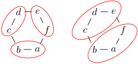
The vertices of Γ/P1 (a 3-clique) and Γ/P2 (a 2-clique) are indicated above by red outlines. There is no consistent transversal of P1 (LHS) because there is no 3-clique subgraph of Γ with one vertex from each set in P1. For Γ/P2 (RHS), ⋔1 = {p′ ↦→ f, p′′ ↦→ e} is a transversal of P2 consistent with Γ, because the subgraph of Γ induced by {e, f} is a 2-clique with one vertex from each of p′ and p′′ .
A transversal of a well-formed ˆ P consistent with Γ(Π) is isomorphic to an instantiation of Π/P consistent with Π. Accordingly, Problem 1 is an instance of the following.
Problem 2. Given Γ, a partition P of V (Γ) and v ∈ V (Γ), is there a consistent transversal of P which covers v?
We now derive the complexity of Problem 2. We first show that the following problem is NP-complete, and use that result to show that Problem 2 is also NP-complete.
Problem 3. Given graph Γ and a partition P of V (Γ), is there a transversal of P consistent with Γ?
Lemma 1. Problem 3 is NP-complete.
Proof. Membership in NP is given because a transversal's consistency can clearly be tested in polynomial-time. We then show the problem is NP-hard by demonstrating a polynomialtime reduction from SAT. Consider SAT problems given by formulae ϕ in conjunctive normal form. Assume every pair of clauses is mutually satisfiable-i.e., for clauses c1, c2 ∈ ϕ, for two literals ℓ1 ∈ c1 and ℓ2 ∈ c2 we have ℓ1 ̸= ¬ℓ2 (when this assumption is violated, unsatisfiability can be decided in polynomial-time). Consider the graph Γ(ϕ), where V (Γ(ϕ)) = {vℓc | c ∈ ϕ, ℓ ∈ c}, and E(Γ(ϕ)) = {{vℓ1c1 , vℓ2c2 } | c1, c2 ∈ ϕ, ℓ1 ∈ c1, ℓ2 ∈ c2, ℓ1 ̸= ¬ℓ2}. Now let P = {{vℓc | ℓ ∈ c} | c ∈ ϕ}. Note that P is a partition of V (Γ(ϕ)) and every set in P corresponds to a clause in ϕ. Because all the clauses in ϕ are mutually satisfiable, the quotient Γ(ϕ)/P is a clique. Now we prove there is a model for ϕ iff there is a transversal of P consistent with Γ(ϕ). (⇒) A model M has the property ∀c ∈ ϕ. ∃ℓ ∈ c. M |= ℓ. Due to the correspondence between sets in P and clauses in ϕ, a transversal ⋔ of P can be constructed by selecting one satisfied literal from each clause. Based on a model, ⋔ will never select conflicting literals. All members of R(⋔) are pairwise connected, so ⋔ is consistent with Γ(ϕ) as required. (⇐) By definition ⋔ is consistent with Γ(ϕ), so the subgraph of Γ induced by R(⋔) is a clique. Let L be literals corresponding to R(⋔), and note that its elements are pairwise consistent. A model M for ϕ is constructed by assigning v to ⊤ where v occurs positively in L, and to ⊥ otherwise.
Theorem 2. Problem 2 is NP-complete.
Proof. Consistency of a transversal ⋔ is clearly polynomialtime testable, as is the coverage condition that v ∈ R(⋔). Thus, we have membership in NP. NP-hardness follows from the following reduction from Problem 3 (P3). Taking P and Γ as inputs to P3, construct the graph Γ′ , where: V (Γ′ ) = V (Γ) ∪ {v}, v an auxiliary vertex; and E(Γ′ ) = E(Γ) ∪ {{v, u} | u ∈ V (Γ)}. There is a solution to P3 with inputs Γ and P iff P2 is soluble with inputs Γ′ , P ∪ {{v}} (= P ′ ) and v. (⇒) If ⋔ is a transversal of P consistent with Γ, then ⋔∪{{v} ↦→ v}(= ⋔′ ) is a transversal of P ′ . As v is fully connected, ⋔′ is consistent with Γ′ . ⋔′ is a solution to P2 because v ∈ R(⋔′ ). (⇐) If ⋔′ is a solution to P2 with inputs Γ′ , P ′ and v, then ⋔′ is a transversal of P ′ , and also P. All edges in E(Γ′ ) are in E(Γ), with the exception of those adjacent v, and since ⋔′ is consistent with Γ′ , then ⋔′ is consistent with Γ. Thus, ⋔′ solves P3.
Note: the NP-hard canonicalisation problem-the optimisation problem posed at each state encountered by orbit search-is not known to be in NP. Our above results imply that exploitation of symmetry via instantiation poses a decision problem in NP that needs to be solved only once.
5 Concrete Plan fromQuotient Plan
Having computed isomorphic subproblems ∆ that cover the goals of Π, a concrete plan is a concatenation of plans for members of ∆. However, this is not always straightforward.
Example 5. Take Π2, P and ⋔ from Example 2. Note ⋔′ = {p1 ↦→ x, p2 ↦→ b, p3 ↦→ n} is also an instantiation of Π2/P consistent with Π2. Observe that {⋔LΠ2/PM, ⋔′ LΠ2/PM} covers the concrete goal G = {m, n}. A plan for Π2/P is ˙π′ = ({p1, p2}, {p3, p1}) and its two instantiations are ⋔L ˙π′ M = ({x, a}, {m, x}) and ⋔′ L ˙π′ M = ({x, b}, {n, x}). Concatenating ⋔L ˙π′ M and ⋔′ L ˙π′ M in any order does not solve Π2 because both plans require x initially, but do not establish it. To overcome this issue in practice, before we solve Π2/P we augment its goal with the assignment p1 ↦→⊤.
We now give conditions under which concatenation is valid, and detail the quotient-goal augmentation step we use to ensure validity in practice. We shall use the well-known notion of projection, where Y ⇂X is a version of Y with all elements mentioning an element not in X removed. 1 In addition, we will write Y ⇂X to mean Y ⇂D(X), for the common case where we wish to project with respect to all the variables in the domain of a problem, state or set of assignments.
Definition 11 (Needed Assignments, Preceding Problem). Needed assignments, N(Π), are assignments in the preconditions of actions and goal conditions that also occur in I, i.e., N(Π) = (pre(A) ∪ G) ∩ I. Problem Π1 is said to precede Π2, written Π1 ▷Π2, iff
- (i) The needed assignments of Π2 which a plan for Π1 could modify occur in G1, and
- (ii) G2 contains all the assignments in G1 which a plan for Π2 might modify.
Example 6. Consider Π2 and Π3 from Examples 2 and 3 respectively. N(Π2) = {x, a, b} and N(Π3) = G1 = {m, n}. Since G2⇂N(Π3) = G2, (I3⇂Π2 )⇂N(Π3) = G2, G2⇂Π3 = G2 and G3⇂Π2 = G2, we have Π2 ▷ Π3.
Writing ˙πi· ˙πj for concatenation of plans ˙πi, ˙πi+1 . . . ˙πj, a simple inductive argument gives the following:
Lemma 2. Let Π1 . . . ΠN be a set of problems satisfying Πj▷ Πk for all j < k ≤ N. For 1 ≤ i ≤ N if state s satisfies Ii ⊆ s and ˙πi solves Πi, then e(s, ˙π1· ˙πN)⇂Gi = Gi.
Take problem Π and a set of problems Π, we say that Π covers Π iff ∀g ∈ G. ∃Π′ ∈ Π. g ∈ G′ and ∀Π′ ∈ Π. Π′ ⊆ Π. I.e., every goal from Π is stated in one or more members of Π, a set of subproblems of Π.
Theorem 3. Consider a set Π1 . . .ΠN of problems that covers Π, satisfying Πj ▷Πk for all j < k ≤ N. For 1 ≤ i ≤ N if ˙πi is a plan for Πi, then ˙π1· ˙πN is a plan for Π.
This theorem follows directly from the fact that the set of problems covers Π and from Lemma 2.
We now address the question: When can plans for a set of isomorphic subproblems be concatenated to provide a concrete plan? We provide sufficient conditions in terms of the concepts of common and sustainable variables.
1 A formal definition was given recently by Helmert et al. (2014).
Definition 12 (Common Variables). For a set of instantiations ∆, the set of common variables, written ⋂v ∆, comprises variables in ⋃⋔∈∆ R(⋔) that occur in the ranges of more than one member of ∆.
Definition 13 (Sustainable Variables). A set of variables V in a problem Π is sustainable iff I⇂V = G⇂V .
Theorem 4. Take problem Π, partition P of D(Π) where the quotient Π/P(= Π′ ) is well-defined, with solution ˙π′ , and consistent instantiations ∆. Suppose {⋔LΠ′ M | ⋔ ∈ ∆}(= Π) covers Π, and QL⋂v ∆M ∩ D(N(Π′ ))-i.e., based on Definition 7, the orbits of common variables from needed assignments-are sustainable in Π′ . Then any concatenation of the plans {⋔L ˙π′ M | ⋔ ∈ ∆} solves Π.
Proof. Identify the elements in ∆ by indices in {1..|∆|}. Let k ∈ {1..|∆|} and Πk = ⋔kLΠ′ M, and note R(⋔k) = D(Πk). Take ⋔i, ⋔j ∈ ∆, where i, j ∈ {1..|∆|} and i ̸= j. We first show that Πi ▷ Πj. For any p ∈ P, ⋔i(p) = ⋔j(p) if ⋔i(p) ∈ R(⋔i) ∩ R(⋔j). Therefore, Ii⇂Πj = Ij⇂Πi and Gi⇂Πj = Gj⇂Πi , providing the right conjunct in Definition 11. For the left conjunct, note D(N(Πj)) ⊆ D(Πj) and D(Πi) ∩ D(Πj) ⊆ ⋂v ∆. The sustainability premise-Q(⋂v ∆) ∩ D(N(Π′ )) is sustainable in Π′-then provides that D(Πi) ∩ D(N(Πj)) is sustainable in Πi-i.e., Ii⇂N(Πj) = Gi⇂N(Πj) . Thus Gi⇂N(Πj) = (Ij⇂Πi )⇂N(Πj) , and we conclude Πi▷Πj . Since a plan ⋔kL ˙π′ M solves ⋔kLΠ′ M, (⋔kLΠ′ M).I ⊆ Π.I, therefore as per Theorem 3 a solution to Π is ˙π1· ˙πN.
In practice we take V ∗ = QL⋂v ∆M ∩ D(N(Π/P)), and augment the goal of the quotient Π/P by adding (Π/P).I⇂V ∗ . Call the resulting problem Πq and its solution ˙πq . Theorem 4 shows that any concatenation of the plans {⋔L ˙πq M | ⋔ ∈ ∆} solves Π. Thus, our approach is sound.
Example 7. Take Π2, P, ⋔ and ⋔′ from Example 5. There is one common variable, {x} = ⋂v ∆ from the orbit {p1} = QL⋂v ∆M. Here N(Π2/P) = {p1, p2}, and the orbit of the common needed variable is {p1} = QL⋂v ∆M ∩ N(Π2/P). To solve Π2 via solving Π2/P, we augment the goal (Π2/P).G with the assignment to p1 in (Π2/P).I. The resulting problem, Πq2 , is equal to Π2/P except that it has the goals Πq2 .G = {p1, p3}. A plan for Πq2 is ˙πq = ({p1, p2}, {p3, p1})({}, {p1}), and two instantiations of it are ⋔L ˙πq M = ({x, a}, {m, x})({}, {x}) and ⋔′ L ˙πq M = ({x, b}, {n, x})({}, {x}). Concatenating ⋔L ˙πq M and ⋔′ L ˙πq M in any order solves Π2.
6 Experimental Results
Implemented in C++, 2 our approach uses: NAUTY\TRACES to calculate symmetries [McKay and Piperno, 2014]; Z3 to find isomorphic subproblems [de Moura and Bjørner, 2008]; and the initial-plan search by LAMA as the base planner [Richter and Westphal, 2010]. We limit base planner runtimes to 30 minutes.
2 bitbucket.org/MohammadAbdulaziz/planning.git in codeBase.
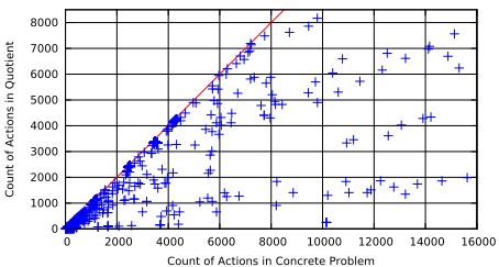
By running our algorithm, we obtained a set of benchmarks with soluble descriptive quotients whose solutions can be instantiated to concrete plans. That set includes 439 problems, from 16 IPC benchmarks and 4 benchmarks from [Porco et al., 2013]. In all our experimentation we identified 120 instances where we were able to confirm that the descriptive quotient does not have a solution and the concrete problem does. Figure 1 plots the sizes, in terms of the number of actions, of concrete and quotient problem descriptions. The plotted data shows that the descriptive quotient can be much smaller than its concrete counterpart. In just over 15% of instances the quotient has less than half the number of actions. Here, we also analyzed what aspects of our approach are computationally expensive. In 79% of cases 99% of the runtime of our approach is executing the base planner. In 96% of cases 95% of the runtime of our approach is executing the base planner. Overall, 3% of time is spent in instantiation and finding chromatic numbers.
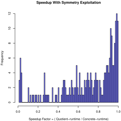
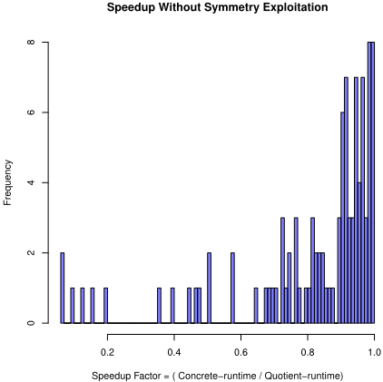
We examined where our approach is comparatively scalable and fast compared to the base planner. For 430 instances where the base planner and our approach are successful, Figure 2 displays the speedup factors where planning via the descriptive quotient is comparatively fast. Overall, for 68% of instances our approach is comparatively fast, and in 15% planning via the quotient is at least twice as fast. With few exceptions, instances where our approach is at least twice as fast are from GRIPPER, HIKING, MPRIME, MYSTERY, PARCPRINTER, PIPESWORLD, TPP and VISITALL. In 5 problems from HIKING, 2 from PARCPRINTER, 1 from TETRIS and 1 from KCOLOURABILITY, the base planner cannot solve the concrete problem, but can solve the quotient. Planning via the quotient can also be slow, primarily due to the extra cost of finding symmetries, 3 and because LAMA is heuristic and occasionally finds that the quotient poses a more challenging problem. Figure 3 provides the dual to Figure 2, showing cases where planning directly for the concrete problem is comparatively fast. This is the case in 32% instances, and indeed in 2% our approach is at least twice as slow.
3 If symmetries are given as part of the problem description, or if one resorts to more heuristic methods of discovering them, such as those described by [Guere and Alami, 2001; Fox and Long, 2002], this burden is relieved.
Finally, it is worth highlighting the difference between searching for a plan in the state-space of the descriptive quotient versus approximate orbit search-i.e., searching for a plan in an approximation of the quotient state-space-as is done in the state-of-the-art techniques for exploiting symmetries in planning. 4 In comparing those approaches, we measure the number of states expanded using a breadth-first search. We consider the IPC instances GRIPPER-20 and MPRIME-21, the largest instances from domains GRIPPER and MPRIME reported solved by Pochter et al. (2011) using breadth-first search. Those authors report the number of states expanded to be 60.5K and 438K, respectively. Using that search to solve the problem posed by our descriptive quotient, we expand 6 and 203K states, respectively.
7 Conclusions, Related and FutureWork
We plan with symmetries using the small descriptive quotient of the concrete problem description. A concrete plan is obtained by concatenating instantiations of the plan for the descriptive quotient. Unlike existing approaches, our search for a plan does not need to reason about symmetries between concrete states and the effects of actions on those. Plan search can be performed by an off-the-shelf SAT/CSP solver, in which case symmetry breaking constraints are not required. Alternatively, using a state-based planner we avoid repeated (approximate) solution to the intractable canonicalisation problem, a clear bottleneck of recent planning algorithms. In this respect, our approach is similar to searching in a counting abstraction, as surveyed by [Wahl and Donaldson, 2010]. That approach treats a transition system isomorphic to the quotient transition system. That system has a state-space which can be exponentially larger than that of a descriptive quotient-i.e., the descriptive quotient will model 1 object, whereas the quotient transition system models N symmetric objects. Existing state-based methods also plan in that relatively large quotient system, and face an additional intractable problem for every encountered state. By employing approximate canonicalisation, such methods face a state-space much larger than that posed by the quotient system, which can be exponentially larger than that posed by a descriptive quotient.
4 Such a comparison is admittedly unfair, as the problem posed by a descriptive quotient is not a bisimulation of the concrete problem.
Our approach decomposes a problem into subproblems, and in that respect is related to factored planning [Amir and Engelhardt, 2003; Brafman and Domshlak, 2006; Kelareva et al., 2007]. There are close ties between factored planning, identifying tractable classes of planning problem, and derivation of tight plan length upper bounds-i.e., in the sense developed in [Rintanen and Gretton, 2013]. We therefore note that (i) the relationship between symmetry and upper bounds has been explored previously, and (ii) symmetries have started to be explored in a factored planning setting. Guere and Alami (2001) propose to plan via a shape-graph, a compact description of the problem state space in which states are represented by equivalence classes of symmetric states. As well as planning by searching in that graph, using the diameter of the shape-graph Guere and Alami are able to calculate tight upper bounds for the highly symmetric GRIPPER and BLOCKS-WORLD domains. Symmetries were explored in factored planning in the context of merge-and-shrink heuristics [Helmert et al., 2014]. Sievers et al. (2015) developed a symmetry guided merging operation which yields relatively compact heuristic models, improving the scalability of that approach. Future research may explore descriptive quotients: to develop heuristics, to characterise tractable classes, and to develop bounding methods.
Acknowledgement
We would like to thank Brendan McKay, Miquel Ram´ırez, Patrik Haslum and Alban Grastien for useful discussions.
@inproceedings{ijcai2015p212,
  title     = {Exploiting Symmetries by Planning for a Descriptive Quotient},
  author    = {Abdulaziz, Mohammad and Norrish, Michael and Gretton, Charles},
  booktitle = {Proceedings of the Twenty-Fourth International Joint Conference on
               Artificial Intelligence, {IJCAI-15}},
  publisher = {International Joint Conferences on Artificial Intelligence},
  editor    = {Qiang Yang and Michael Wooldridge},
  pages     = {1479--1485},
  year      = {2015},
  month     = {7},
  note      = {Main Track},
  url       = {https://ijcai.org/proceedings/2015/212},
}
TY - CPAPER TI - Exploiting Symmetries by Planning for a Descriptive Quotient AU - Abdulaziz, Mohammad AU - Norrish, Michael AU - Gretton, Charles T2 - Proceedings of the Twenty-Fourth International Joint Conference on Artificial Intelligence, IJCAI-15 PB - International Joint Conferences on Artificial Intelligence PY - 2015 SP - 1479 EP - 1485 UR - https://ijcai.org/proceedings/2015/212 ER -Copied
Machine-readable versions of this paper, for tools and AI agents:





