
Convolutional Neural Networks for Text Hashing
Proceedings of the Twenty-Fourth International Joint Conference on Artificial Intelligence. Main Track. Pages 1369-1374.
© 2015 International Joint Conferences on Artificial Intelligence
Abstract
Hashing, as a popular approximate nearest neighbor search, has been widely used for large-scale similarity search. Recently, a spectrum of machine learning methods are utilized to learn similarity-preserving binary codes. However, most of them directly encode the explicit features, keywords, which fail to preserve the accurate semantic similarities in binary code beyond keyword matching, especially on short texts. Here we propose a novel text hashing framework with convolutional neural networks. In particular, we first embed the keyword features into compact binary code with a locality preserving constraint. Meanwhile word features and position features are together fed into a convolutional network to learn the implicit features which are further incorporated with the explicit features to fit the pre-trained binary code. Such base method can be successfully accomplished without any external tags/labels, and other three model variations are designed to integrate tags/labels. Experimental results show the superiority of our proposed approach over several state-of-the-art hashing methods when tested on one short text dataset as well as one normal text dataset.
- [Andoni and Indyk, 2006] Alexandr Andoni and Piotr Indyk. Near-optimal hashing algorithms for approximate nearest neighbor in high dimensions. In FOCS, pages 459-468, 2006.
- [Blunsom et al., 2014] Phil Blunsom, Edward Grefenstette, Nal Kalchbrenner, et al. A convolutional neural network for mod- elling sentences. In ACL, 2014.
- [Cachopo, 2007] Ana Margarida de Jesus Cardoso Cachopo. Im- proving Methods for Single-label Text Categorization. PhD thesis, Universidade Técnica de Lisboa, 2007.
- [Collobert et al., 2011] Ronan Collobert, Jason Weston, Léon Bottou, Michael Karlen, Koray Kavukcuoglu, and Pavel Kuksa. Natural language processing (almost) from scratch. JMLR, 12:2493-2537, 2011.
- [Gong et al., 2013] Yunchao Gong, Svetlana Lazebnik, Albert Gordo, and Florent Perronnin. Iterative quantization: A pro- crustean approach to learning binary codes for large-scale im- age retrieval. TPAMI, 35(12):2916-2929, 2013.
- [Hu et al., 2014] Baotian Hu, Zhengdong Lu, Hang Li, and Qingcai Chen. Convolutional neural network architectures for matching natural language sentences. In NIPS, pages 2042- 2050, 2014.
- [Lai et al., 2015] Siwei Lai, Liheng Xu, Kang Liu, and Jun Zhao. Recurrent convolutional neural networks for text clas- sification. In AAAI, 2015.
- [Lin et al., 2013] Guosheng Lin, Chunhua Shen, David Suter, and Anton van den Hengel. A general two-step approach to learning-based hashing. In ICCV, pages 2552-2559. IEEE, 2013.
- [Lin et al., 2014] Guosheng Lin, Chunhua Shen, Qinfeng Shi, Anton van den Hengel, and David Suter. Fast supervised hash- ing with decision trees for high-dimensional data. In CVPR, pages 1971-1978. IEEE, 2014.
- [Liu et al., 2012] Wei Liu, Jun Wang, Rongrong Ji, Yu-Gang Jiang, and Shih-Fu Chang. Supervised hashing with kernels. In CVPR, pages 2074-2081. IEEE, 2012.
- [Lu et al., 2014] Shixiang Lu, Zhenbiao Chen, and Bo Xu. Learning new semi-supervised deep auto-encoder features for statistical machine translation. In ACL, volume 1, pages 122- 132, 2014.
- [Manku et al., 2007] Gurmeet Singh Manku, Arvind Jain, and Anish Das Sarma. Detecting near-duplicates for web crawling. In WWW, pages 141-150. ACM, 2007.
- [Mikolov et al., 2013] Tomas Mikolov, Ilya Sutskever, Kai Chen, Greg S Corrado, and Jeff Dean. Distributed represen- tations of words and phrases and their compositionality. In NIPS, pages 3111-3119, 2013.
- [Pennington et al., 2014] Jeffrey Pennington, Richard Socher, and Christopher D Manning. Glove: Global vectors for word representation. EMNLP, 12, 2014.
- [Phan et al., 2008] Xuan-Hieu Phan, Le-Minh Nguyen, and Susumu Horiguchi. Learning to classify short and sparse text & web with hidden topics from large-scale data collections. In WWW, pages 91-100. ACM, 2008.
- [Salakhutdinov and Hinton, 2009] Ruslan Salakhutdinov and Geoffrey Hinton. Semantic hashing. International Journal of Approximate Reasoning, 50(7):969-978, 2009.
- [Shen et al., 2014] Yelong Shen, Xiaodong He, Jianfeng Gao, Li Deng, and Grégoire Mesnil. Learning semantic representa- tions using convolutional neural networks for web search. In WWW, pages 373-374. International World Wide Web Con- ferences Steering Committee, 2014.
- [Turian et al., 2010] Joseph Turian, Lev Ratinov, and Yoshua Bengio. Word representations: a simple and general method for semi-supervised learning. In ACL, pages 384-394, 2010.
- [Wang et al., 2013a] Qifan Wang, Lingyun Ruan, Zhiwei Zhang, and Luo Si. Learning compact hashing codes for ef- ficient tag completion and prediction. In CIKM, pages 1789- 1794. ACM, 2013.
- [Wang et al., 2013b] Qifan Wang, Dan Zhang, and Luo Si. Se- mantic hashing using tags and topic modeling. In SIGIR, pages 213-222. ACM, 2013.
- [Weiss et al., 2009] Yair Weiss, Antonio Torralba, and Rob Fer- gus. Spectral hashing. In NIPS, pages 1753-1760, 2009.
- [Xia et al., 2014] Rongkai Xia, Yan Pan, Hanjiang Lai, Cong Liu, and Shuicheng Yan. Supervised hashing for image re- trieval via image representation learning. In AAAI, 2014.
- [Zeng et al., 2014] Daojian Zeng, Kang Liu, Siwei Lai, Guangyou Zhou, and Jun Zhao. Relation classification via convolutional deep neural network. In COLING, pages 2335- 2344, 2014.
- [Zhang and Li, 2014] Dongqing Zhang and Wu-Jun Li. Large- scale supervised multimodal hashing with semantic correla- tion maximization. In AAAI, 2014.
- [Zhang et al., 2010a] Dell Zhang, Jun Wang, Deng Cai, and Jin- song Lu. Extensions to self-taught hashing: Kernelisation and supervision. practice, 29:38, 2010.
- [Zhang et al., 2010b] Dell Zhang, Jun Wang, Deng Cai, and Jin- song Lu. Laplacian co-hashing of terms and documents. In Advances in Information Retrieval, pages 577-580. Springer, 2010.
- [Zhang et al., 2010c] Dell Zhang, Jun Wang, Deng Cai, and Jin- song Lu. Self-taught hashing for fast similarity search. In SIGIR, pages 18-25. ACM, 2010.
- [Zhang et al., 2013] Debing Zhang, Genmao Yang, Yao Hu, Zhongming Jin, Deng Cai, and Xiaofei He. A unified ap- proximate nearest neighbor search scheme by combining data structure and hashing. In IJCAI, pages 681-687. AAAI Press, 2013. IJCAI
References were extracted automatically from the PDF and may contain errors.
Full text extracted automatically from the PDF; figures, tables and equations may differ. The PDF is the version of record.
1 Introduction
Due to computational and storage efficiencies of compact binary codes, hashing methods have been widely used for Approximate Nearest Neighbors (ANN) search, which is an essential component in a variety of large-scale machine learning problems, such as information retrieval [Zhang et al., 2013], near-duplicates detection [Manku et al., 2007], tag prediction [Wang et al., 2013a], cross-view similarity search [Zhang and Li, 2014], etc.
The existing hashing methods can be roughly divided into two categories: data-oblivious and data-aware. The former, such as famous Locality-Sensitive Hashing (LSH) [Andoni and Indyk, 2006], is useful for the case without preassigned training dataset, while we focus on the latter which can be further divided into three streams. The first stream is unsupervised method [Salakhutdinov and Hinton, 2009; Weiss et al., 2009; Zhang et al., 2010c; Gong et al., 2013], where only unlabeled data is used to learn hash functions. The other two streams are semi-supervised and supervised methods [Zhang et al., 2010a; Liu et al., 2012; Wang et al., 2013b; Lin et al., 2014], in which the tags/labels are exploited to guide hash function learning.
The key problem is that the most existing hashing methods directly embed texts into a low-dimension binary space from the explicit feature space, such as word-count vectors and term frequency-inverse document frequency (TF-IDF) vectors, which usually fail to fully preserve the semantic similarity. For example, there are two texts "President write his first computer program" and "Obama kick off hour of code", hashing methods based on the explicit features cannot see the similarity between the keyword features "President" and "Obama" or "program" and "code". In order to address this problem, some researchers introduce latent semantic approaches to construct similarity relationship in the implicit feature space, such as Latent Dirichlet Allocation (LDA) [Wang et al., 2013b], Latent Semantic Analysis (LSA) and Restricted Boltzmann Machines (RBM) [Salakhutdinov and Hinton, 2009]. Although these methods can capture semantic features, they are still trained based on bag-of-words (BoW) and ignore the contextual information or word order.
Recently, a promising way to alleviate this problem is word embedding and Deep Neural Networks (DNN). With the help of word embedding, true meaningful syntactic and semantic regularities can be captured, and DNN has been proved to be efficient in terms of constructing text representations [Lai et al., 2015]. Recently, Convolutional Neural Networks (CNN), applying convolving filters to local features, have achieved a better performance in many Neural Language Processing (NLP) applications, such as sentence modeling [Blunsom et al., 2014], semantic matching [Hu et al., 2014], web search [Shen et al., 2014] and other traditional NLP tasks [Collobert et al., 2011]. Despite the fact that these works with CNN and word embedding prove a solid success in many NLP tasks, most of themmainly focus on short texts or sentence level datasets and do not always outperform TF-IDF on normal texts in practice.
Besides, word position may result in different meanings on the same term. For example, the word "code", as a noun term, usually exists in the ends of one sentence, meanwhile the verb term usually exists in the middle of one sentence. And text length, playing an important role in semantic match [Lu et al., 2014], should also be utilized for text hashing.
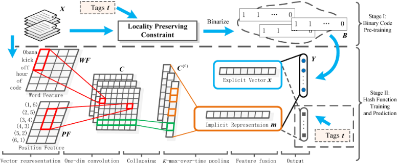
Inspired by all these, in this paper, we aim at addressing the above problems and systematically exploring the power of text hashing via convolutional neural networks. An overall architecture of the proposed Text Hashing with Convolutional neural networks (abbr. to THC) is illustrated in Figure 1, which has two stages. In stage I, we first embed the original features X into binary code B with a locality preserving constraint. Meanwhile, we extract word vectors WF and position vectors PF by looking up word embeddings and position embeddings, and then feed them into a convolutional neural network to learn the implicit representation. Before the output layer, the implicit feature m is integrated with the explicit vector x, TFIDF used in this paper. Finally, we treat the pre-trained code B as the supervision to learn the CNN model which can generate the optimal hash code Y. This is the proposed base model THC-I which is unsupervised, without any external tags/labels at all. If the external tags/labels are available, we integrate these supervised information in stage I and II respectively, and get three supervised variants THC-II, THC-III and THC-IV as described in Figure 1.
Our main contributions are three-fold: 1). We propose a flexible framework, CNN for text hashing, which is able to accommodate both unlabeled and labeled texts. To our best knowledge, this is the first time to exploit CNN to solve text hashing systematically. 2). Besides word embeddings, we also encode the relative distances of each word to the two ends of one text into vectors (referred as position features in this paper) which both include word position and the text length information, and we design a collapsing operation following one-dimensional convolution to couple word features and position features which show further improvement in our experiments. 3). We adapt a simple but effective method by directly incorporating the implicit features and the explicit features to address the limitation that the works via CNN do not always work well on normal texts. Meanwhile, we test and verify experiments on two publicly available text datasets. The experimental results indicate that our approaches can achieve better performances compared with the state-of-the-art methods on both short text dataset and normal text dataset.
2 RelatedWork
Hashing As described before, hash-based methods can be mainly divided into two categories. One category is dataoblivious hashing. As the most popular hashing technique, Locality-Sensitive Hashing (LSH) [Andoni and Indyk, 2006] based on random projection has been widely used for similarity search. However, they do not aware of data distribution, which may lead to generating quite inefficient hash codes in practice [Zhang et al., 2010a]. Recently, more researchers focus attention on the other category, data-aware hashing, by using machine learning algorithms. For example, the Spectral Hashing (SpH) [Weiss et al., 2009] generates compact binary codes by forcing the balanced and uncorrelated constraints into the learned codes. Iterative Quantization (ITQ) [Gong et al., 2013] reduce the dimensionality of input data and binarizes the outcome through minimizing the quantization error. Self-Taught Hashing (STH) [Zhang et al., 2010c] is a method which decomposes the learning procedure into two steps: generating binary code and learning hash function. A supervised version of STH is proposed in [Zhang et al., 2010a] denoted as STHs. Inspire of these methods, Lin et al. [2013; 2014] design a two-step hashing framework (TSH) and use decision trees as hash function in a fast supervised hashing (FastHash). However, the previous hashing methods, directly working in keyword feature space, usually fail to fully preserve semantic similarity for text hashing due to the sparseness of text representations.
Neural Networks Recently, there is a revival of interest in DNN. Among this upsurge, there are two classes of most related works to our work, one is word embedding, and the other is DNN for hashing. For the former, in NLP, more and more tasks have got promising results based on word embeddings, which is primarily based on learning a distributed representation for each word. There are some famous word embeddings. The skip-gram and continuous bag-of-words models of [Mikolov et al., 2013] propose a simple singlelayer architecture based on the inner product between two word vectors. Pennington et al. [2014] introduce a new model for word representation, called GloVe, which captures the global corpus statistics. For the latter, there are two most related works, one is [Salakhutdinov and Hinton, 2009] which uses deep auto encoder to learn hash codes by assuming that the top hidden layer only contains binary units. During the fine-tuning procedure, they use backpropagation to find codes that are good at reconstructing the word-count vector. In the other one, Xia et al. [2014] proposed an image hashing via representation learning, which nevertheless is quite different from NLP tasks. And to our best knowledge, our work is the first time to systematically explore the power of CNN for text hashing with the help of word embeddings.
3 AlgorithmDescription
As described in Figure 1. Given a dataset of n training texts denoted as: X = {x1, x2..., xn} ∈ Rd×n , where d is the dimensionality of the keyword feature. Denote their tags as: t = {t1, t2..., tn} ∈ {0, 1}c×n , where c is the total number of possible tags associated with each text. A tag with label 1 means a text is associated with a certain tag, while a tag with label 0 means a missing tag or the text is not associated with that tag. The goal of THC is to obtain the optimal hash code Y = {y1, y2..., yn}T ∈ {-1, 1}n×r , and a hash function f : Rd → {-1, 1}r , which embeds the query text xq to its compact hash code yq with r bits (r ≪ d). To achieve the similarity-preserving property, we require the similar texts to have similar binary codes in Hamming space.
3.1 Binary Code Pre-training
In this stage, we pre-train binary code B based on the keyword features with a locality preserving constraint, and choose Laplacian affinity loss, also used in [Weiss et al., 2009; Zhang et al., 2010c]. Although many other types of loss functions can be utilized (e.g., KSH [Liu et al., 2012], ITQ [Gong et al., 2013], FastHash [Lin et al., 2014]), a comparison of those loss functions is beyond the scope of this paper. The optimization can be written as:
where Sij is the pairwise similarity between texts xi and xj, and ‖·‖F is the Frobenius norm. The problem is relaxed by discarding B ∈ {-1, 1}n×r , and the r-dimensional real-valued vectors ˜B can be learned from Laplacian Eigenmap. Then, we get the binary code B via the media vector m = median(˜B). In particular, we construct the n × n local similarity matrix S by using heat kernel as follows:
where, σ is a tuning parameter (default is 1), Nk(x) represents the set of k-nearest-neighbors of x and cij is an adjustment coefficient. For THC-I and THC-III, we fix cij to 1, while for THC-II and THC-IV, we set cij a higher value a if two texts xi and xj share a common tag/label and we set cij a lower value b if xi and xj do not share any tag/label. In our experiments, we consistently set the a = 1 and b = 0.1.
3.2 Hash Function Training and Prediction
Learned Features
- Word Representation. Each input word wi is transformed into a vector WFi ∈ Rdw by looking up word embedding E(W) which is a distributed representation of a word. Since there are many high-quality trained word embeddings that are freely available [Turian et al., 2010; Collobert et al., 2011; Mikolov et al., 2013; Pennington et al., 2014]. This work directly chooses these word embeddings and further give a simple comparison in Section 5.2.
- Position Representation. As the input text in Figure 1, the relative distance of the word "code" to the two ends of the text is (6,1) which both include word position and the text length information. We also encode the relative distance into a vector features PFi ∈ Rdp (referred as position features) by looking up position embedding E(p) which is randomly initialized and suitable for the input of neural networks.
Convolutional Neural Networks
- Convolution. By combining the learned features WF and PF, each word is represented as XFi = [WFi,PFi] ∈ R(dw+dp) , and the text matrix is constructed as S = [XFT1 , ...,XFTt ]T ∈ Rt×(dw+dp) , where t is the token number in one text. In this paper, we apply a one-dimensional convolution of the wide type W ∈ Rw×(dw+dp)×n1 to S, where w is the filter width and n1 is the size of feature maps. For convenience, we introduce the matrix of diagonals to indicate the j-th convolutional filter:
After the j-th one-dimensional convolution, we get a resulting matrix Cj ∈ R(t+w-1)×(dw+dp) , generated from a window of embedding features by:
where,
- Collapsing. Since we use one-dimensional convolution, word feature and position feature are independent until now. In order to couple these two features, we introduce a simple operation called collapsing. For the j-th resulting matrix Cj , collapsing directly compresses the dimension (dw+dp) to one. After the collapsing layer, the feature matrix Cj is compressed into a vector C(0) j , and
- Pooling. When a K-max-over-time pooling is applied over the j-th feature vector C(0) j , the K highest values ˆC(0) j are selected. Then, we apply a non-linear operation and select the tanh activation function to ˆC(0) = [ˆC(0) 1 , ..., ˆC(0) n1 ] as follows:
where, m ∈ Rn1K is an implicit semantic vector.
| - | Methods | SearchSnippets | 20Newsgroups | ||||||
|---|---|---|---|---|---|---|---|---|---|
| mP@50 | mP@100 | mP@150 | mP@200 | mP@50 | mP@100 | mP@150 | mP@200 | ||
| THC-II | 79.89 | 79.24 | 78.54 | 77.77 | 79.49 | 78.07 | 76.75 | 75.92 | |
| THC-III | 79.32 | 78.67 | 78.00 | 77.27 | 66.21 | 64.02 | 62.11 | 60.31 | |
| THC-IV | 80.56 | 79.90 | 79.21 | 78.50 | 79.53 | 78.13 | 76.80 | 75.96 | |
| Supervised | TSH-KSH | 71.09 | 70.87 | 70.76 | 70.34 | 75.83 | 75.74 | 75.57 | 75.24 |
| FastHash | 61.23 | 60.97 | 60.52 | 60.22 | 73.76 | 73.54 | 73.34 | 73.17 | |
| STHs | 69.31 | 68.39 | 67.27 | 66.05 | 77.78 | 76.80 | 75.26 | 73.23 | |
| Unsupervised THC-I | 78.07 | 77.46 | 76.80 | 76.08 | 65.83 | 63.73 | 61.82 | 60.03 | |
| STH-RBF | 68.94 | 67.51 | 66.38 | 65.18 | 63.82 | 61.82 | 59.88 | 57.95 | |
| STH | 65.44 | 63.70 | 62.45 | 61.24 | 63.63 | 61.16 | 58.98 | 56.88 | |
| ITQ | 35.03 | 33.24 | 31.73 | 30.45 | 48.31 | 46.55 | 44.87 | 43.17 | |
| LCH | 54.20 | 52.36 | 51.09 | 50.05 | 32.75 | 30.41 | 28.89 | 27.69 | |
| SpH | 32.74 | 29.47 | 27.28 | 25.72 | 32.81 | 27.84 | 24.85 | 22.78 | |
- Output. At the last layer of CNN, we integrate the implicit feature m with the explicit keyword features x ∈ Rd by a linear transformation:
where, α is a combination coefficient, O(H) ∈ Rr is the output vector, WZ ∈ Rr×n1K and WO ∈ Rr×d are weight matrices. To binary the output for hash code representation Y and fit the pre-trained binary code B, we apply r logistic operations to O(H) as follows:
Additionally, for THC-III and THC-IV, we add c output units which correspond to the tags of the training texts. Correspondingly, an additional output vector is given by:
where, O(C) ∈ Rc is the output vector, W′Z ∈ Rc×n1K andW′O ∈ Rc×t are weight matrices. In order to match the tags/labels t, we apply c logistic operations to the additional output vector O(C) as follows:
Backpropagation Training
All of the parameters to be trained are defined as:
Given the training text collection X, the pre-trained binary code B and the tags/labels t, the log likelihood of the parameters can be written down as follows:
We maximize the log likelihood using stochastic gradient descent to compute the optimal parameter θ:
After backpropagation training, we can obtain the optimal hash code Y for the training texts and the network parameter θ. Given a query text xq, we can get its hash code yq by computing the hash function f(xq|θ). Then, the similarity search can be conducted by exploring the Hamming ball volume around the probe query yq.
4 Datasets and Experimental Setup
4.1 Datasets
We test our algorithms on two public text datasets, and the summary statistics of the datasets are described in Table 2.
SearchSnippets 1 . This dataset was selected from the results of web search transaction using predefined phrases of 8 different domains [Phan et al., 2008]. We do not remove any stop words or symbols in the text.
20Newsgroups. We select the popular bydata version and use the stemmed version 2 pre-processed by Ana CardosoCachopo [2007], and we further remove the texts with length more than 300.
For these datasets, we denote the category labels as tags, generate vocabulary from the training sets and randomly select 10% of the training data as the development set.
| Dataset | C | Train/Test | L(mean/max) | |V | |
| Snippets | 8 | 10060/2280 | 17.3/38 | 26265 |
| 20News | 20 | 10443/6973 | 92.8/300 | 41877 |
4.2 Pre-trainedWord Vectors
By default, our experiments ultilize the GloVe embeddings 3 trained by Pennington et al. [2014] on 6 billion tokens of Wikipedia 2014 and Gigaword 5. We also give some comparisons with other word embeddings, such as Senna embeddings 4 [Collobert et al., 2011] and even initialized randomly embeddings. The coverage of these embeddings on two datasets are listed in Table 4, and the words not present in the set of pre-trained words are initialized randomly.
1 http://jwebpro.sourceforge.net/data-web-snippets.tar.gz.
2 http://web.ist.utl.pt/acardoso/datasets/.
3 http://nlp.stanford.edu/projects/glove/.
4 http://ml.nec-labs.com/senna/.
| - | Feature Sets | SearchSnippets | 20Newsgroups | ||||||
|---|---|---|---|---|---|---|---|---|---|
| THC-I | THC-II | THC-III | THC-IV | THC-I | THC-II | THC-III | THC-IV | ||
| Imp. Fea. | WF | 75.34 | 76.76 | 76.59 | 78.11 | 56.09 | 68.50 | 57.94 | 69.64 |
| +PF | 76.21 | 78.03 | 77.75 | 78.87 | 56.52 | 69.60 | 59.04 | 70.03 | |
| Exp. Fea. | TF-IDF | 68.65 | 69.96 | 69.00 | 70.34 | 60.29 | 72.80 | 60.35 | 72.85 |
| Combination | All | 77.46 | 79.24 | 78.67 | 79.90 | 63.73 | 78.07 | 64.02 | 78.13 |
| Other word | All (Senna) | 75.11 | 75.27 | 75.16 | 75.69 | 63.52 | 77.98 | 63.64 | 77.98 |
| embeddings | All (rand) | 65.78 | 68.31 | 65.96 | 68.37 | 63.50 | 77.84 | 63.67 | 77.83 |
| Dataset | GloVe | Senna | ||
|---|---|---|---|---|
| |V | | |T | | |V | | |T | | |
| Snippets | 18301 | 201147 | 16249 | 196748 |
| (69%) | (94%) | (61%) | (91%) | |
| 20News | 20793 (49%) | 1317799 (81%) | 16300 (38%) | 1246474 (77%) |
4.3 Comparisons
Eight widely used hashing methods compared with our methods are Spectral Hashing (SpH) [Weiss et al., 2009], Laplacian Co-Hashing (LCH) [Zhang et al., 2010b], SelfTaught Hashing (STH) [Zhang et al., 2010c], STH with RBF (STH-RBF) [Zhang et al., 2010a], Iterative Quantization (ITQ) [Gong et al., 2013], the supervised version of STH (STHs) [Zhang et al., 2010a], Two Step Hashing with KSH and RBF (TSH-KSH) [Lin et al., 2013] and Fast Supervised Hashing (FastHash) [Lin et al., 2014]. The former five methods do not used any tags, and the later three methods utilize tag information. The results of all baseline methods are obtained by the open-source implementation provided on their corresponding author's homepage. For ITQ, we use LDA 5 to reduce dimensions of original features to 512 due to the dimensionality curse. Note that we do not select Semantic Hashing (SH) [Salakhutdinov and Hinton, 2009] as a comparison because that SH has been surpassed by the baseline method SpH [Weiss et al., 2009].
In order to evaluate our approach's performance, mean precision of top N retrieved texts (mP@N) based on Hamming distance ranking is used throughout the paper as a main criteria, which is also used in [Zhang et al., 2013; Lin et al., 2013; Wang et al., 2013b]. For the original keyword feature space cannot well reflect the semantic similarity, even worse for short texts, we simply test if the two texts share any common tag/label to decide whether a semantic similar text. This methodology is used in [Salakhutdinov and Hinton, 2009; Zhang et al., 2010c; Wang et al., 2013b]. The results reported are the average of 5 trials.
5 http://jgibblda.sourceforge.net/: -alpha 0.5 -beta 0.1.
4.4 Hyperparameter Settings
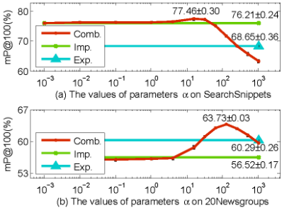
In our experiments, the most of parameters are set uniformly for these datasets. The parameter k in Equation 2 is fixed to 7 when constructing the graph Laplacians in our approach, as well as in the baseline methods, STH, STH-RBF and STHs. We set the width of the convolutional filter w as 3, the size of feature map n1 as 80, the value of K in max pooling layer as 2, the dimension of word embeddings dw as 50, the dimension of position embeddings dp as 8 and the learning rate λ as 0.01. Moreover, the feature weight α at the output layer are tuned through the grid from 0.001 to 1024. The optimal weights are α = 16 on SearchSnippets and α = 128 on 20Newsgroups.
5 Results and Analysis
5.1 Comparison Experiments
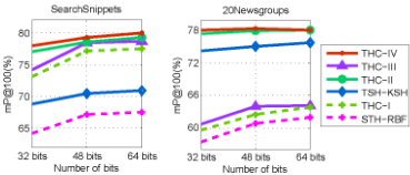
Table 1 shows the mP@N results of our THC and other comparison methods on two text datasets. We can see that our base method THC-I significantly outperform these unsupervised baseline methods about 9%-10%/2%-3% on SearchSnippets/20Newsgroups. Compared with the supervised baseline methods, THC-II and THC-IV also give a better performance. THC-IV is the most effective method and THC-II is better than THC-III in most situations. Furthermore, THC-I even achieves a better performance than these supervised baseline methods on SearchSnippets, but does not achieve the same effect on 20Newsgroups. The possible reason is that some topics of the 20Newsgroups are very closely related to each other (e.g. comp.sys.ibm.pc.hardware/ comp.sys.mac.hardware) [Wang et al., 2013b], which cause confusion to the methods without utilizing any external tags. Meanwhile, Figure 2 shows the mP@100 results with various length of hash bits. The results indicate that our methods, both supervised approaches (solid line in Figure 2) and unsupervised ones (dashed line), get consistent improvement compared with the corresponding baselines in all the cases, except the case of THC-III on 20Newsgroups. In fact, THC-III's performance is almost the same as unsupervised ones, such as THC-I, in the case of 20Newsgroups. It seems that the external tags/labels do not show the expected effect, and why? An explanation maybe that the way in which the hash approaches use the external tags/labels is count. Specifically, from Figure 1, we know that for THC-IV and THC-II as well as STH-KSH, the tags/labels are used in the stage I, while for THC-III, the tags/labels are used in the stage II. So we guess that not only whether or not to use the external label, but also that where and how to use the tags/labels, maybe even more important for improving hashing's performance.
5.2 Influence of Learned Features
In this experiment, we study the effect of the implicit features learned from word features and position features, and the explicit features, TF-IDF. The mP@100 results are presented in Table 3. By adding position feature, the proposed methods achieve consistently, approximately 1%-2%, improvements compared with only using word embeddings. Further, by adding the explicit features, the performance further improve about 1%-2%/5%-7% on SearchSnippets/20Newsgourps. Explicit features give a more remarkably performance's improvement on 20Newsgroups than on SearchSnippets. The reason may be that Searchsnippets is a short text dataset, for which the implicit features rather than the explicit features is more useful for alleviating the sparsity problem, while 20Newsgroups is a normal text dataset, for which the effect of explicit features is more useful. And when we combine the implicit features with the explicit features together, we get the best performance. For the same reason above, we can see that pretrained word embeddings, such as GloVe embedding (default used in our methods) and Senna Embedding, are more useful for our methods to get a better performance, compared with random initialized ones, especially on shorter text dataset.
5.3 Influence of Hyperparameters
Here, we first study the performance of THC with respect to the combination coefficient α. We tune the parameter α from 0.001 to 1024 and report the results on two datasets in Figure 3. It is clear that the combination of implicit feature and explicit feature get the best performance on two text datasets consistently, although the specific optimal values of α are sightly different. Meanwhile, when α is set to a small value, implicit features contribute more to the performance, and when α is set to a large value, explicit feature give more contribution. The result indicates that implicit features contribute more in the case of short text, and explicit ones do more in the case of normal text. The reason is the same as Table 3 analysed in Section 5.2.
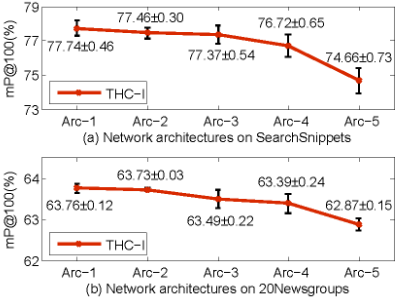
For CNN architecture, we fix the word dimension, learning rate and the width of the convolutional filters following previous studies [Collobert et al., 2011; Zeng et al., 2014]. Moreover, we fix the number of neurons at the layer of implicit representation to 160 just for easily giving some compared network structures as listed in Table 5, and the results are illustrated in Figure 4. We can see that the performances on two datasets almost unchange when the parameter K in the max pooling layer is smaller than 4. Meanwhile, the more maps at the convolutional layer, the more computational complexity, and Arc-2 used in this paper is a good trade-off.
| - | Arc-1 | Arc-2 | Arc-3 | Arc-4 | Arc-5 |
|---|---|---|---|---|---|
| Maps num. | 160 | 80 | 40 | 20 | 10 |
| K-max | 1 | 2 | 4 | 8 | 16 |
6 Conclusion
In this paper, we design a text hashing via convolutional neural network. The implicit features learned from CNN and the explicit features extracted from the raw texts are successfully integrated for hashing task. We also propose a collapsing operation following one-dimensional convolution to couple word features and position features, and the influence of the learned features are further evaluated in the experiments. And the experimental results on two text datasets indicate that the proposed approaches achieve remarkable improvements. For the future work, as our approach has exhibited a promising results, we guess that it has a potential to further improve the performance by exploring some sophisticated neural networks to model normal texts.
Acknowledgments
We thank anonymous reviewers for their comments, and this work was supported by the National Basic Research Program of China (No. 2012CB316300), the National Natural Science Foundation of China (No. 61203281, No. 61303172, No. 61403385) and the Hundred Talents Program of Chinese Academy of Sciences (No. Y3S4011D31).
@inproceedings{ijcai2015p197,
  title     = {Convolutional Neural Networks for Text Hashing},
  author    = {Xu, Jiaming and Wang, Peng and Tian, Guanhua and Xu, Bo and Zhao, Jun and Wang, Fangyuan and Hao, Hongwei},
  booktitle = {Proceedings of the Twenty-Fourth International Joint Conference on
               Artificial Intelligence, {IJCAI-15}},
  publisher = {International Joint Conferences on Artificial Intelligence},
  editor    = {Qiang Yang and Michael Wooldridge},
  pages     = {1369--1374},
  year      = {2015},
  month     = {7},
  note      = {Main Track},
  url       = {https://ijcai.org/proceedings/2015/197},
}
TY - CPAPER TI - Convolutional Neural Networks for Text Hashing AU - Xu, Jiaming AU - Wang, Peng AU - Tian, Guanhua AU - Xu, Bo AU - Zhao, Jun AU - Wang, Fangyuan AU - Hao, Hongwei T2 - Proceedings of the Twenty-Fourth International Joint Conference on Artificial Intelligence, IJCAI-15 PB - International Joint Conferences on Artificial Intelligence PY - 2015 SP - 1369 EP - 1374 UR - https://ijcai.org/proceedings/2015/197 ER -Copied
Machine-readable versions of this paper, for tools and AI agents:





