
Revisiting Gaussian Process Dynamical Models
Proceedings of the Twenty-Fourth International Joint Conference on Artificial Intelligence. Main Track. Pages 1047-1052.
© 2015 International Joint Conferences on Artificial Intelligence
Abstract
The recently proposed Gaussian process dynamical models (GPDMs) have been successfully applied to time series modeling. There are four learning algorithms for GPDMs: maximizing a posterior (MAP), fixing the kernel hyperparameters α_ (Fix.α_), balanced GPDM (B-GPDM) and two-stage MAP (T.MAP), which are designed for model training with complete data. When data are incomplete, GPDMs reconstruct the missing data using a function of the latent variables before parameter updates, which, however, may cause cumulative errors. In this paper, we present four new algorithms (MAP+, Fix.α+, B-GPDM+ and T.MAP+) for learning GPDMs with incomplete training data and a new conditional model (CM+) for recovering incomplete test data. Our methods adopt the Bayesian framework and can fully and properly use the partially observed data. We conduct experiments on incomplete motion capture data (walk, run, swing and multiple-walker) and make comparisons with the existing four algorithms as well as k-NN, spline interpolation and VGPDS. Our methods perform much better on both training with incomplete data and recovering incomplete test data.
- [An et al., 2012] B. An, H. K, and F. C. Park. Grasp motion learn- ing with Gaussian process dynamic models. In Proceedings of IEEE International Conference on Automation Science and En- gineering, pages 1114-1119, 2012.
- [Chen et al., 2009] J. Chen, M. Kim, Y. Wang, and Q. Ji. Switch- ing Gaussian process dynamic models for simultaneous compos- ite motion tracking and recognition. In Proceedings of IEEE Conference on Computer Vision and Pattern Recognition, pages 2655-2662, 2009.
- [Dallaire et al., 2009] P. Dallaire, C. Besse, S. Ross, and B. Chaib- draa. GP-POMDP: Bayesian reinforcement learning in con- tinuous POMDPs with Gaussian processes. In Proceedings of IEEE/RSJ International Conference on Intelligent Robots and Systems, pages 2604-2609, 2009.
- [Damianou et al., 2011] A. C. Damianou, M. K. Titsias, and N. D. Lawrence. Variational Gaussian process dynamical systems. Advances in Neural Information Processing Systems, 24:2510- 2518, 2011.
- [Deena and Galata, 2009] S. Deena and A. Galata. Speech-driven facial animation using a shared Gaussian process latent variable model. In Proceedings of the 5th International Symposium on Advances in Visual Computing, pages 89-100, 2009.
- [Deena et al., 2013] S. Deena, S. Hou, and A. Galata. Visual speech synthesis using a variable-order switching shared Gaus- sian process dynamical model. IEEE Transactions on Multime- dia, 15:1755-1768, 2013.
- [Gamage et al., 2011] N. Gamage, T. C. Kuang, R. Akmeliawati, and S. Demidenko. Gaussian process dynamical models for hand gesture interpretation in sign language. Pattern Recognition Let- ters, 32:2009-2014, 2011.
- [Henter et al., 2012] G. E. Henter, M. R. Frean, and W. B. Kleijn. Gaussian process dynamical models for nonparametric speech representation and synthesis. In Proceedings of IEEE Interna- tional Conference on Acoustics, Speech and Signal Processing, pages 4505-4508, 2012.
- [Li et al., 2013] W. Li, J. Sun, X. Zhang, and Y. Wu. Spatial constraints-based maximum likelihood estimation for human motions. In Proceedings of IEEE International Conference on Signal Processing, Communication and Computing, pages 1-6, 2013.
- [Park and Yoo, 2011] H. Park and C. D. Yoo. Gaussian process dynamical models for phoneme classification. In Proceedings of Neural Information Processing System Workshop on Bayesian Nonparametrics: Hope or Hype, pages 1-2, 2011.
- [Raskin et al., 2008] L. Raskin, E. Rivlin, and M. Rudzsky. Us- ing Gaussian process annealing particle filter for 3D human tracking. EURASIP Journal on Advances in Signal Processing, 2008:1-13, 2008.
- [Sun, 2013] S. Sun. A review of deterministic approximate infer- ence techniques for Bayesian machine learning. Neural Com- puting and Applications, 23:2039-2050, 2013.
- [Taubert et al., 2012] N. Taubert, A. Christensen, D. Endres, and M. A. Giese. Online simulation of emotional interactive be- haviors with hierarchical Gaussian process dynamical models. In Proceedings of the ACM Symposium on Applied Perception, pages 25-32, 2012.
- [Urtasun et al., 2006] R. Urtasun, D. J. Fleet, and P. Fua. 3D peo- ple tracking with Gaussian process dynamic models. In Proceed- ings of IEEE Computer Society Conference on Computer Vision and Pattern Recognition, pages 238-245, 2006.
- [Urtasun et al., 2007] R. Urtasun, D. J. Fleet, and N. D. Lawrence. Modeling human locomotion with topologically constrained la- tent variable models. In Proceedings of IEEE International Con- ference on Computer Vision Workshop on Human Motion: Un- derstanding, Modeling, Capture and Animation, pages 104-118, 2007.
- [Urtasun et al., 2008] R. Urtasun, D. J. Fleet, A. Geiger, J. Popović, T. J. Darrell, and N. D. Lawrence. Topologically- constrained latent variable models. In Proceedings of the 25th International Conference on Machine Learning, pages 1080- 1087, 2008.
- [Velychko et al., 2014] D. Velychko, D. Endres, N. Taubert, and M. A. Giese. Coupling Gaussian process dynamical models with product-of-experts kernels. In Proceedings of the 24th Inter- national Conference on Artificial Neural Networks, pages 1-9, 2014.
- [Wang et al., 2006] J. M. Wang, D. J. Fleet, and A. Hertzmann. Gaussian process dynamical models. Advances in Neural Infor- mation Processing Systems, 19:1441-1448, 2006.
- [Wang et al., 2008a] J. Wang, Y. Yin, and H. Man. Multiple hu- man tracking using particle filter with Gaussian process dynam- ical model. EURASIP Journal on Image and Video Processing, 2008:1-10, 2008.
- [Wang et al., 2008b] J. M. Wang, D. J. Fleet, and A. Hertzmann. Gaussian process dynamical models for human motion. IEEE Transactions on Pattern Analysis and Machine Intelligence, 30:283-398, 2008.
- [Wang, 2013] Z. Wang. Intention Inference and Decision Mak- ing with Hierarchical Gaussian Process Dynamics Models. PhD thesis, Darmstadt University of Technology, 2013.
References were extracted automatically from the PDF and may contain errors.
Full text extracted automatically from the PDF; figures, tables and equations may differ. The PDF is the version of record.
1 Introduction
The Gaussian process dynamical model (GPDM) was recently proposed by augmenting the Gaussian process latent variable model with a GP prior to model sequential motion data and predict the latent positions [Wang et al., 2006]. It provides a nonlinear probabilistic mapping from latent positions to human poses and a nonlinear dynamical mapping on the latent space. Wang et al. [2008b] described and compared four algorithms for learning GPDMs: maximizing a posterior (MAP), fixing the kernel hyperparameters ¯α (Fix.¯α), balanced GPDM (B-GPDM) and two-stage MAP (T.MAP).
GPDMs are widely applicable to sequential data analysis such as people tracking, motion data recognition and synthesis and computer animation. For example, Urtasun et al. [2006] introduced the balanced GPDM method for learning smooth prior models of human poses and motions for 3D people tracking. Park and Yoo [2011] used the GPDM for phoneme classification. Gamage et al. [2011] employed the GPDM as an alternative to hidden Markov models and artificial neural networks for hand gesture recognition in the context of sign language translation. Henter et al. [2012] introduced the GPDM for speech representation and synthesis. An et al. [2012] presented an online method for grasping motion learning using the GPDM.
Some variants and extensions of GPDMs have also been developed to adapt to specific applications. For human tracking, the particle filter GPDM was proposed, which can improve the stability and robustness of tracking [Raskin et al., 2008] and deal with multi-target tracking [Wang et al., 2008a]. For trajectory prediction, GPDMs were adapted to learn effective representations of the environment dynamics in continuous partially observable Markov decision processes [Dallaire et al., 2009]. For modeling multiple activities, back constraints and topological constraints were incorporated within the local linear GPDM [Urtasun et al., 2007; 2008]. In order to account for multiple types of dynamics, Chen et al. [2009] proposed to combine switching models with GPDMs to produce a switching GPDM, which has a switching layer on top of the latent variables. Similarly, the switching shared GPDM (SSGPDM) which is a nonparametric switching state-space model was proposed by Chen et al. [2009]. It is an extension of the shared GPDM [Deena and Galata, 2009], where multiple shared GPDMs are indexed by switching states. Later, Deena et al. [2013] used SSGPDM with a variable-order Markov model on phonemes for visual speech synthesis. In order to learn the interactions between pairs of actors, a hierarchical model based on GPDMs referred as HGPDM was devised by Taubert et al. [2012]. Similarly, Wang [2013] incorporated the exogenous variables in GPDMs, resulting in an HGPDM which achieves improved interpretation, analysis, and prediction of human movements. Recently, Velychko et al. [2014] presented an approach to coupling GPDMs based on a product-of-experts, which is capable to learn different motion styles of body parts for movement design and recombine previously learned component dynamics for complex coordinated movements.
As introduced above, GPDMs and their variants are widely used in practical applications. But unfortunately, data obtained from the real world are often incomplete. For example, in medical problems, not all patients have the needed measurements. In the optical motion capture problem, parts of data can get lost as a result of some factors such as occlusions, limited field of view, errors in the capturing process or faults in the capturing equipment. Therefore, addressing missing data in GPDMs has great significance and practical value. The existing methods for learning GPDMs were almost all designed for complete training data. When the training data are incomplete, a simple reconstruction was usually adopted before parameter updates [Wang et al., 2006], which is likely to bring cumulative errors. What's more, most literatures about GPDMs [Wang et al., 2006; 2008b; Li et al., 2013] only dealt with the situation in which some data subsequences are totally missing. This is just one specific situation of data incompleteness. In practice, there are different situations of data incompleteness. For example, if we use a matrix to represent multiple-output sequential data, the situations include row missing, column missing and block missing. Our work is to address missing data in GPDMs where the data incompleteness can be in any situation and the missing data can occur in the training or (and) test set. In this paper, the Bayesian framework is adopted. No matter which situation of data incompleteness, for training, Bayesian methods can be used to maximize the posterior of unknown variables conditional on the observed data. Similarly, if the test data are incomplete, the lost data can be recovered by maximizing the posterior distribution of the conditional model given the observed test data and the learned model. This idea was employed before, e.g., in reconstructing the parts of motion capture data with the variational Gaussian process dynamical system (VGPDS) [Damianou et al., 2011].
In this paper, we revisit GPDMs in different situations of data incompleteness and develop four algorithms (MAP+, Fix.¯α+, B-GPDM+ and T.MAP+) for training GPDMs with incomplete data and a conditional model (CM+) for recovering the incomplete test data. The highlights of our work are summarized as follows. Firstly, the proposed approaches can fully and properly use the partially observed data while the existing work reconstructs the missing data using a function of the latent variables, which may cause cumulative errors. Therefore, the proposed approaches are promising to provide significant improvements. In our experiments on the human motion data, the lost parts of the body in the sequences are recovered more accurately, as expected. Secondly, the proposed approaches for GPDMs can handle various complex situations of data incompleteness while most exiting work on GPDMs can only deal with very simple situations. In view of all the different situations of data incompleteness, our approaches show advantages for recovering missing data.
2 Review of GPDMs
GPDMs were proposed to analyze sequential data. Let Y = [y1, ..., yN]⊤ be the data in the observation space and X = [x1, ..., xN]⊤ be the variables in the latent space where yi ∈ RD and xi ∈ Rd . The likelihood of Y given X is expressed as a product of GPs (one for each of the D data dimensions)
where W is a scaling diagonal matrix and KY is an N ×N kernel matrix constructed by a kernel function κY with parameters ¯ β = {βi}3i=1 : κY (x, x′ ) = β1exp(- β2 2 ||x - x′ ||2 ) + β-1 3 δx,x′ . The distribution of X is given by a firstorder Markov Gaussian process
where X2:N = [x2, ..., xN]⊤, KX is a kernel matrix constructed from [x1, ..., xN-1]⊤, and x1 has an isotropic Gaussian prior. The GPDM uses a "linear+RBF" kernel for KX with parameters ¯α = {αi}4i=1 : κX(x, x′ ) = α1exp(- α2 2 ||x - x′ ||2 ) + α3x⊤x′ + α-1 4 δx,x′ . The priors of the kernel hyperparamters are placed with p(¯α) ∝ ∏i α-1 i and p( ¯ β) ∝ ∏i β-1 i . Parameter W has a broad half-normal prior, p(W) = ∏Dm=1 2 σ√2π exp(- w2m 2σ2 ), where wm > 0 corresponds to the diagonal elements of W and σ is often fixed 1 .
Then, the joint probability distribution of latent variables, observations, and parameters is given by
Note that, Y can represent multiple sequences Y (1) , ..., Y (P) , with lengths N1, ...,NP . Then X2:N is composed of the associated latent variables X(1) , ...,X(P) as X2:N = [X(1)⊤ 2:N1 , ...,X(P)⊤ 2:NP ]⊤ and X1:N-1 is given by X1:N-1 = [X(1)⊤ 1:N1-1 , ...,X(P)⊤ 1:NP -1 ]⊤.
2.1 GPDMLearning
The existing learning algorithms for GPDMs include MAP, Fix.¯α, B-GPDM and T.MAP [Wang et al., 2008b]. The first three algorithms are based on MAP and the fourth uses Monte Carlo EM (MCEM). MAP based methods require minimizing the joint negative log-posterior of the unknowns
-lnp(X, ¯α, ¯ β,W|Y ) expressed as L + const, where const represents a constant and
with
MAP Parameters and latent variables are optimized through minimizing (3) with respect to W in a closed form and with respect to {X, ¯α, ¯ β} alternately using the scaled conjugate gradient method (SCG).
Fix. ¯α Hyperparamters ¯α are fixed as [0.009, 0.2, 0.001,106 ]⊤ instead of being optimized to ensure that p(X|¯α) represents a strong preference for smooth observation sequences. B-GPDM B-GPDM was introduced by multiplying LX in
1 It is set to 103 in our experiments as inWang et al. [2008b].
Algorithm 1 MAP+ estimation of {X, ¯α, ¯ β, W }.
Require: Data {Y:,cd, Ycn,md}, integers {d, I, J}. Initialize Xcn with PCA on Ycn,: with d dimensions. Initialize Xmn using the NN 2 or cubic spline 3 method. Initialize ¯α← (0.9, 1, 0.1, e), ¯ β ← (1, 1, e), {wk} ← 1. 1: for i =1 to I do 2: for j in cd do 3: w2 j ←N(Y ⊤ :,jK-1 Y Y:,j + 1 σ2 )-1 4: end for 5: for j inmd do 6: w2 j ← Nc(Y ⊤ cn,jK-1 Ycn Ycn,j + 1 σ2 )-1 7: end for 8: {X, ¯α, ¯ β} ← optimize (7) using SCG for J iterations. 9: end for(3) by a coefficient Dd to balance the influences of the observation reconstruction error in the high dimensional space and the prediction error in the low dimensional latent space before optimization. As a result, B-GPDM adapts the objective function (3) to favor smooth latent variable sequences.
T.MAP Unlike the previous learning algorithms, T.MAP uses MCEM to optimize Θ = {¯α, ¯ β,W} and MAP to optimize X. In the E-step of MCEM, the expected complete negative log likelihood -lnp(Y,X|Θ) under p(X|Y,Θi ) is approximately computed by LE(Θ) ≈ - 1R ∑Rr=1 lnp(Y,Xr |Θ), where {Xr }Rr=1 ∼ p(X|Y,Θi ) are sampled using hybrid Monte Carlo (HMC). In the M-step, the hyperparameters Θi+1 are optimized by minimizing LE(Θ). As the second stage, given the optimized Θi+1 , X is optimized through maximizing ln p(X, Θi+1 |Y ) with SCG.
2.2 Conditional GPDM
Given the learned GPDM Γ = {Y,X, ¯α, ¯ β,W}, which includes the observations, learned latent variables and parameters, one can optimize the latent variables corresponding to a new observation sequence with a conditional GPDM (CM). In addition, one can predict or generate a new sequence only with an initial value x1.
In the CM, the distribution over a new sequence Y ∗ ∈ RM×D and its associated latent variable X∗ ∈ RM×d conditional on Γ is given by
2 NN is short for 1-nearest neighbor where for each frame the values of known dimensions are compared to each example in the present data to find the closest match, which is used in S2 and S3.
3 Cubic spline [Wang et al., 2008b] is a kind of interpolation method relying on the data before and after the missing data, which is used in S1.
Algorithm 2 T.MAP+ estimation of {X, ¯α, ¯ β, W }.
Require: Data {Y:,cd, Ycn,md}. Integers {d,R, I, J,K}. Initialize Xcn with PCA on Ycn,: with d dimensions. Initialize Xmn using the NN or cubic spline method. Initialize ¯α← (0.9, 1, 0.1, e), ¯ β ← (1, 1, e), {wk} ← 1. 1: for i =1 to I do 2: Generate {Xr }Rr=1 ∼ p(X|Y:,cd, Ycn,md, ¯α, ¯ β,W) using HMC sampling. 3: Construct {KrY ,KrYcn ,KrX} from {Xr }Rr=1. 4: for j = 1 to J do 5: for k in cd do 6: w2 j ←N(Y ⊤ :,k 1R ∑Rr=1 (KrY )-1Y:,k + 1 σ2 )-1 7: end for 8: for k in md do 9: w2 j ← Nc(Y ⊤ cn,k 1R ∑Rr=1 (KrYcn )-1Ycn,k+ 1 σ2 )-1 10: end for 11: {¯α, ¯ β} ←optimize ˜ LE (Θ) using SCG for K iterations. 12: end for 13: X ←maximize lnp(X, ¯α, ¯ β, W |Y:,cd, Ycn,md). 14: end forHere, p(X∗ |Γ) is calculated as
where ZX = X∗ 2:N - C ⊤K-1 X X2:N and KX∗ = D - C ⊤K-1 X C. (C)ij = κX(xi, x∗j ) and (D)ij = κX(x∗i , x∗j ) are the elements of the (N-P)×(M-1) and (M-1)×(M1) kernel matrices, respectively. p(Y ∗ |X∗ , Γ) is calculated as
where ZY = Y ∗ - A⊤K-1 Y Y and KY ∗ = B -A⊤K-1 Y A. (A)ij = κY (xi, x∗j ) and (B)ij = κY (x∗i , x∗j ) are the elements of the N×M and M×M kernel matrices, respectively.
To optimize the latent variables associated with new sequences, one can obtain X∗ by maximizing (6). To predict or generate a new sequence given x1, one can first set the latent variable at each time step to be the most likely (mean) value given the previous set as µX(xt-1) = kX(xt-1)⊤K-1 X X2:N. Then reconstruct the new data in the observation space by the mean function µY (x∗ ) = kY (x∗ )⊤K-1 Y Y .
2.3 GPDMwith Incomplete Data
It is indeed possible for GPDMs to deal with missing data [Wang et al., 2008b]. However, no matter for incomplete training or test data, these methods use the mean function µY (X) introduced above to reconstruct the missing data. This reconstruction procedure would be performed before optimizing (3) or (6), respectively. Moreover, the reconstruction uses the latent variables obtained by some initialization methods. Thus the performance of these methods is quite limited and large cumulative errors may be incurred.
3 Our Methods
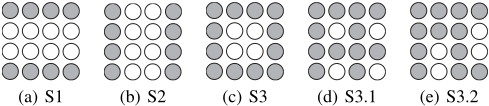
We summarize data incompleteness into three situations, i.e., row missing (S1), column missing (S2) and block missing
| 07 01 | 35 01 | 35 18 | 64 01 | four-walker | |
|---|---|---|---|---|---|
| NN | 15.72 / · | 7.24 / · | 40.70 / · | 24.06 / · | 14.00 / · |
| MAP | 15.72 / 59.89 | 6.57 / 2.50 | 33.87 / 3.00 | 20.76 / 0.66 | 17.34 / 9.59 |
| Fix. ¯α | 15.34 / 88.70 | 6.42 / 2.00 | 35.17 / 3.32 | 19.48 / 0.48 | 17.81 / 6.13 |
| B-GPDM | 14.45 / 5.42 | 5.97 / 0.57 | 27.01 / 0.31 | 17.07 / 0.22 | 13.47 / 0.24 |
| T.MAP | 14.91 / 19.79 | 6.89 / 2.57 | 23.15 / 1.74 | 14.90 / 1.74 | 12.15 / 10.19 |
| MAP+ | 14.33 / 3.71 | 6.26 / 0.07 | 24.99 / 0.27 | 12.80 / 0.14 | 13.91 / 2.72 |
| Fix. ¯α+ | 15.34 / 2.49 | 6.08 / 0.10 | 28.92 / 0.42 | 15.27 / 0.16 | 16.69 / 2.07 |
| B-GPDM+ | 14.38 / 1.47 | 6.51 / 0.27 | 26.68 / 0.26 | 16.06 / 0.17 | 15.43 / 0.19 |
| T.MAP+ | 15.37 / 4.38 | 6.62 / 0.37 | 18.00 / 0.20 | 14.68 / 0.34 | 10.77 / 2.44 |
(S3) in Figures 1(a), 1(b) and 1(c), where the gray nodes are observed and the white are unobserved. We first give the definitions of some symbols: mn with length Nm represents the time indices of missing data, and md with length Dm represents the dimension indices of missing data. Correspondingly, cn and cd with lengths Nc and Dc are the complements of mn and md in the whole indices [1 : N] and [1 : D], respectively. Thus, the missing data can be expressed as Ymn,md and the present data can be expressed as Ycn,md, Y:,cd. In particular, Figure 1(a) can be expressed as row missing; Figure 1(b) can be expressed as column missing; Figure 1(c) can be expressed as block missing in which mn = [2, 3], md = [2, 3], cn = [1, 4] and cd = [1, 4].
It is worth noting that Figures 1(a) and 1(b) are two specific cases of Figure 1(c), and Figure 1(c) can be extended to any situations of data incompleteness. A complex situation is that the missing data are non-contiguous over time or dimensions. We divide this case of data incompleteness into two situations as in Figures 1(d) and 1(e), and note that a) if the missing data can be formed into a matrix, the methods for reconstruction are the same as the methods for addressing missing data that are contiguous over time and dimensions; b) otherwise, the missing data should be divided into blocks. We first give methods for both training and testing with incomplete data in the case of S3. After that, we will explain how to adapt our methods to the situation of non-contiguously missing.
3.1 GPDMwith Incomplete Training Data
The GPDMs are defined as before, and now suppose the training data are incomplete as in Figure 1(c). According to the Bayesian framework, the joint distribution of the latent variables, the observed data and the parameters are given by
where Xcn means the cnth rows of X and Wmd represents a diagonal matrix whose diagonal elements are the mdth diagonal elements of W. In this case we propose four new learning methods for GPDM training, which are denoted MAP+, Fix.¯α+, B-GPDM+ and T.MAP+. In MAP based methods, the GPDMwith incomplete data is learned through minimizing the joint negative log-posterior of the unknowns
-lnp(X, ¯α, ¯ β, W |Y:,cd, Ycn,md) which is given, up to an additive constant, by
with
Here, LX has the same formulation as (5). We give the details for MAP+, Fix.¯α+, B-GPDM+ and T.MAP+ below. MAP+ Parameters are optimized through minimizing (7) with respect to W in a closed form and with respect to {X, ¯α, ¯ β} alternately using SCG. The detailed procedure is described in Algorithm 1. We set d = 3, I = 100 and J = 10 in our experiments.
Fix.¯α+ Hyperparamters ¯α in (7) are fixed as [0.009, 0.2, 0.001, 106 ]⊤ instead of being optimized.
B-GPDM+ Similar to B-GPDM, LX in (7) is multiplied by
a coefficient Dd to balance the objective terms in the GPDM. T.MAP+ T.MAP+ has the same principle as T.MAP, which uses MCEM to optimize Θ = {¯α, ¯ β,W} and MAP to optimize X. Since the data are now incomplete, some calculations are different. In the E-step of MCEM, the expected joint negative log-likelihood -lnp(Y:,cd, Ycn,md,X|Θ) under p(X|Y:,cd, Ycn,md,Θi ) is approximately computed by ˜ LE(Θ) ≈ - 1R ∑Rr=1 lnp(Y:,cd, Ycn,md,Xr |Θ), where {Xr }Rr=1 ∼ p(X|Y:,cd, Ycn,md,Θi ) are sampled using HMC. In the M-step, the hyperparameters Θi+1 are optimized by minimizing ˜ LE(Θ). As the second stage, given the optimized Θi+1 , X is optimized through maximizing lnp(X,Θi+1 |Y:,cd, Ycn,md) by SCG. The detailed procedure is given in Algorithm 2. We set d = 3, R = 50, I = 10, J = 10 and K = 10 in our experiments.
Comparing Algorithms 1 and 2 with the existing algorithms [Wang et al., 2008b], we find that the proposed methods only double the computational complexities in the worst case. Moreover, reconstructions for missing data before parameter updates disappear in the proposed methods, which will reduce the time cost. Further, when data are incomplete as in S1, the proposed methods would be more efficient.
3.2 GPDMwith Incomplete Test Data
We present a new conditional model (CM+) to recover the missing test data Y ∗mn,md ∈ RMm×Dm. In the CM+, defining ˜ Y = [Y ⊤, Y ∗⊤ cn,: ]⊤, ˜ Y ∗ = Y ∗mn,: , ˜X = [X⊤,X∗⊤ cn ]⊤ and
˜X∗ = X∗mn, the posterior density of Y ∗mn,md is
where ˜ ZY = Y ∗mn,md - ˜ A⊤K-1 ˜ Y ˜ Y:,md and K˜ Y ∗ = ˜B - ˜ A⊤K-1 ˜ Y ˜ A. ( ˜ A)ij = κY (˜xi, ˜x∗j ) and ( ˜B)ij = κY (˜x∗i , ˜x∗j ) are the elements of the (N +Mc)×Mm and Mm×Mm kernel matrices, respectively. Different from the previous CM, the optimal value of X∗ is obtained by maximizing the joint conditional distribution of observed test data Y ∗ :,cd, Y ∗ cn,md and the associated latent variable X∗ given the learned model Γ
With X∗ optimized, the mean function µ˜ Y ( ˜X∗ ) = k˜ Y ( ˜X∗ )⊤K-1 ˜ Y ˜ Y is used for recovering the lost test data.
3.3 Non-contiguouslyMissing
Recall that Figure 1(c) can be extended to more complex situations in which the missing data are non-contiguous over time or dimensions as exhibited in Figures 1(d) and 1(e). Our approaches can be applied to these situations with some reformulations or minor modifications. Specifically, for S3.1 the approaches presented above do not require modifications but with md = [2, 4], mn = [2, 4], cd = [1, 3] and cn = [1, 3]. For S3.2, the missing data can be expressed as md1 = [2], mn1 = [3, 4], md2 = [4] and mn2 = [2, 3]. The complement indices are: cn1 = [1, 2], cn2 = [1, 4] and cd = [1, 3]. Note that cd includes the complements of the union set of md1 and md2 in the whole indices [1 : D]. Since data on different dimensions are conditionally independent, the corresponding likelihood of Ycn,md is replaced by the product of the likelihoods of Ycn1,md1 and Ycn2,md2 . We then only need to adjust (7) and (10) accordingly.
4 Experiments
The benchmark data used for experiments are human motion capture data from the Carnegie Mellon University motion capture database. As in Wang et al. [2008b], we use a specific version of the default skeleton in the database for which each pose is 50-dimensional. To evaluate the effectiveness of the proposed methods, two different types of experiments have been performed: training with incomplete data and recovering incomplete test data.
4.1 Training with Incomplete Data
We evaluate the proposed four learning algorithms for handling incomplete training data. The data used include two single-walker sequences 07 01.amc (1-2-260/50-100/1-38) 4 and 35 01.amc (55-4-338/41-60/7-31), a single-runner sequence 35 18.amc (1-2-160/21-50/23-48), a single-swinger sequence 64 01.amc (120-4-400/16-40/7-31) and a fourwalker sequence spliced by 35 02.amc (55-4-338/16-40/138), 10 04.amc (222-4-499/16-40/1-38), 12 01.amc (22-4328/16-40/1-38) and 16 15.amc (62-4-342/16-40/1-38). In a word, these incomplete data are all in S3. Note that, the missing data in the four-walker sequence are non-contiguous over time. For each kind of motion data, we perform the four proposed learning algorithms MAP+, Fix.¯α+, B-GPDM+ and T.MAP+ compared with MAP, Fix. ¯α, B-GPDM and T.MAP, as well as NN. Moreover, we repeat all the experiments on each motion data for nine times with different missing data. That is, mn and md slide on three different windows, respectively. For example, for 07 01, mn = [50 : 100], [51 : 101] or [52 : 102] andmd = [1 : 38], [2 : 39] or [3 : 40].
Table 1 shows the averaged root mean square error (RMSE) per missing frame and the averaged negative logposterior (-LP) over the missing data. All the shown -LPs in this paper are the actual -LPs divided by 100. The best results are marked in bold for each motion sequence. Through the table, we see that the lowest RMSE and -LP are almost all obtained by the proposed algorithms. Further, the four proposed algorithms outperform MAP, Fix.¯α, B-GPDM and T.MAP on most sequences, respectively. Note that, since the data in some frames are not completely lost, the present data on some known dimensions will help to learn the model. In this case, the dynamics of the model are not the unique factor to influence the performance of the model. This explains why Fix.¯α+, B-GPDM+ and T.MAP+ which favor smooth latent trajectories do not always perform best.
4 "1-2-260/50-100/1-38" means that the data are downsampled from frames 1 to 260 by a factor of 2, with mn = [50 : 100] and md = [1 : 38].
| 35 03 | 12 02 | 16 21 | 12 03 | 07 01 | 07 02 | 08 01 | 08 02 | AVG. | |
|---|---|---|---|---|---|---|---|---|---|
| k-NN | 40.64 / · | 40.36 / · | 49.91 / · | 50.45 / · | 78.81 / · | 64.40 / · | 76.48 / · | 77.06 / · | 59.76 / · |
| VGPDS | 49.92 / 12.29 | 45.72 / 10.84 | 36.00 / 7.47 | 43.20 / 10.32 | 75.74 / 24.24 | 73.23 / 23.37 | 88.78 / 14.75 | 71.92 / 12.29 | 60.56 / 14.45 |
| MAP+CM | 37.26 / 3.06 | 43.42 / 78.44 | 36.18 / 6.11 | 46.55 / 3.46 | 74.33 / 5.41 | 68.05 / 2.87 | 85.61 / 4.95 | 64.77 / 17.88 | 57.02 / 15.27 |
| Fix. ¯α+CM | 51.58 / 4.98 | 50.24 / 5.31 | 39.96 / 2.77 | 56.69 / 7.24 | 82.55 / 7.75 | 80.32 / 7.01 | 96.20 / 10.79 | 65.65 / 8.12 | 65.40 / 6.75 |
| B-GPDM+CM | 46.72 / 4.71 | 50.15 / 7.74 | 42.33 / 3.83 | 53.57 / 8.14 | 83.02 / 13.40 | 76.08 / 12.02 | 90.04 / 14.66 | 65.40 / 7.45 | 63.41 / 8.99 |
| T.MAP+CM | 57.04 / 2.26 | 59.60 / 2.62 | 46.96 / 8.13 | 58.59 / 3.19 | 86.81 / 6.97 | 88.56 / 6.44 | 93.93 / 8.25 | 66.20 / 19.59 | 69.71 / 7.18 |
| MAP+CM+ | 34.56 / 1.10 | 43.34 / 1.45 | 36.32 / 1.85 | 42.92 / 1.65 | 71.51 / 2.50 | 66.53 / 1.16 | 81.18 / 2.19 | 67.75 / 6.12 | 55.52 / 2.25 |
| Fix. ¯α+CM+ | 50.08 / 5.02 | 49.99 / 5.35 | 40.17 / 2.79 | 56.82 / 7.22 | 82.66 / 7.58 | 79.49 / 7.15 | 95.63 / 11.05 | 65.77 / 8.16 | 65.08 / 6.79 |
| B-GPDM+CM+ | 46.72 / 4.71 | 50.15 / 7.74 | 42.33 / 3.83 | 53.57 / 8.14 | 83.02 / 13.40 | 76.08 / 12.02 | 90.04 / 14.66 | 65.40 / 7.45 | 63.41 / 8.99 |
| T.MAP+CM+ | 56.86 / 1.06 | 57.88 / 1.60 | 48.77 / 2.90 | 60.24 / 1.92 | 85.03 / 1.87 | 83.29 / 2.00 | 94.88 / 4.74 | 70.05 / 7.45 | 69.63 / 2.94 |
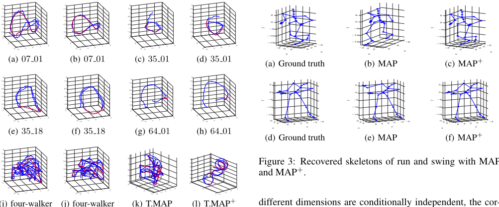
Figure 2 shows the 3D latent trajectories learned from incomplete data, in which from (a) to (j), the couples of figures with the same name are the 3D trajectories of the same data learned by MAP on the left and MAP+ on the right, respectively. Figures 2(k) and 2(l) are the 3D trajectories of the four-walker motion data learned by T.MAP and T.MAP+, respectively. The red line corresponds to the missing frames and the blue line corresponds to the present frames. From the figure we can find that the latent trajectories learned through MAP+ are much smoother than those through MAP. This is because MAP+ makes full use of the data on the known dimensions while learning the dynamics of the latent trajectories. However, the simple reconstruction approach in MAP makes it rely on the old latent variables too much, which leads to cumulative errors. In Figures 2(i) and 2(j), the motion data combining four walkers are not well learned by MAP or MAP+, which is consistent to the conclusions in Wang et al. [2008b]. In addition, Wang et al. [2008b] showed that for complete data the walk cycles from the four subjects learned with T.MAP are smooth and separated in the latent space. However, when the data are incomplete (as shown in Figures 2(k) and 2(l)), T.MAP cannot achieve the same effects while T.MAP+ can.
In order to show the correctness of the recovery more intuitively, we exhibit the recovered skeletons of run and swing on a certain frame with MAP and MAP+ in Figure 3. Obviously, the legs of the runner and the right arm of the swinger are not recovered well by MAP. But, the skeletons recovered by MAP+ and the ground truth are almost the same.
4.2 Recovering Incomplete Test Data
Now we consider the tasks of filling in lost parts of new data in two situations (S1 and S2) of data incompleteness. We perform the proposed conditional model CM+ and the existing conditional model CM to recover the missing test data. The learned GPDMs on the four-walker motion data using different learning algorithms are employed. For clarity, we define the approaches as "learning algorithm + CM+" and "learning algorithm + CM".
| Complete training data | Incomplete training data | ||
|---|---|---|---|
| Methods | AVG. | Methods | AVG. |
| k-NN | 50.46 / · | k-NN | 70.01 / · |
| spline | 122.24 / · | spline | 122.24 / · |
| MAP+CM | 53.69 / 230.73 | MAP+CM | 57.13 / 847.46 |
| Fix. ¯α+CM | 46.55 / 3.54 | Fix. ¯α+CM | 56.72 / 3.43 |
| B-GPDM+CM | 51.52 / 4.50 | B-GPDM+CM | 52.63 / 6.42 |
| T.MAP+CM | 50.90 / 158.17 | T.MAP+CM | 51.26 / 505.02 |
| MAP+CM+ | 51.73 / 186.19 | MAP++CM+ | 51.83 / 229.88 |
| Fix. ¯α+CM+ | 46.54 / 3.53 | Fix.¯α++CM+ | 50.87 / 2.66 |
| B-GPDM+CM+ | 51.42 / 4.41 | B-GPDM++CM+ | 52.91 / 3.69 |
| T.MAP+CM+ | 51.04 / 70.56 | T.MAP++CM+ | 49.05 / 107.96 |
First we consider the column missing case. Eight 50-frame sequences with 40 dimensions removed are taken to be recovered. The training data used here are complete so that the learning algorithms for GPDMs combined with CM+ are the same to those for GPDMs combined with CM. The experiments are performed for three times with the same setting but with md = [1 : 40], [2 : 41] and [3 : 42] for each time, respectively. Table 2 gives the averaged results in terms of the RMSE of recovering and -LP of missing data over three experiments. Besides GPDM based methods, VGPDS and kNN are also employed for comparisons. Here, k is set to 15 as in Wang et al. [2008b] where they tried k=[3, 6, 9, 15, 20], with 15 giving the lowest average error. We do not include spline which is only suitable in S1. The VGPDS which assumes that sequences are independent cannot get as good performance as GPDMs on the current data. The proposed CM+ recovers the missing parts more accurately than the existing CM. Moreover, MAP+CM+ performs best because the current situation of data incompleteness is that data on some dimensions are missing from the start to the end of a sequence: Other algorithms relying too much on the dynamics of the model cannot help to recover missing data well in this situation.
In order to verify the versatility of our methods, we also conduct experiments on recovering test data with some interval frames missing. In this situation, we consider two cases in which the training data are complete and incomplete, respectively. For incomplete training data, GPDMs are learned by the existing and proposed algorithms, respectively. VGPDS
which doesn't handle this situation is not compared. Experiments on the same sequences as Table 2 are performed, in which missing frames are [5 : 35]. Due to the limited space, the averaged RMSE and -LP over all the test sequences are presented in Table 3. Fix.¯α+CM+ and T.MAP++CM+ perform best with complete and incomplete training data, respectively. The methods which favor the dynamics perform better than MAP+CM+ because data in all dimensions before and after the missing frames are given in these experiments.
5 Conclusions
In this paper, we have proposed four learning algorithms (MAP+, Fix.¯α+, B-GPDM+ and T.MAP+) for training GPDMs with incomplete training data and a condition model (CM+) for recovering incomplete test data. The approaches were developed under the Bayesian framework [Sun, 2013]. The advantages of the proposed approaches have been demonstrated for different situations of data incompleteness.
Acknowledgments
The corresponding author Shiliang Sun would like to thank supports from the National Natural Science Foundation of China under Project 61370175, and Shanghai Knowledge Service Platform Project (No. ZF1213).
@inproceedings{ijcai2015p152,
  title     = {Revisiting Gaussian Process Dynamical Models},
  author    = {Zhao, Jing and Sun, Shiliang},
  booktitle = {Proceedings of the Twenty-Fourth International Joint Conference on
               Artificial Intelligence, {IJCAI-15}},
  publisher = {International Joint Conferences on Artificial Intelligence},
  editor    = {Qiang Yang and Michael Wooldridge},
  pages     = {1047--1052},
  year      = {2015},
  month     = {7},
  note      = {Main Track},
  url       = {https://ijcai.org/proceedings/2015/152},
}
TY - CPAPER TI - Revisiting Gaussian Process Dynamical Models AU - Zhao, Jing AU - Sun, Shiliang T2 - Proceedings of the Twenty-Fourth International Joint Conference on Artificial Intelligence, IJCAI-15 PB - International Joint Conferences on Artificial Intelligence PY - 2015 SP - 1047 EP - 1052 UR - https://ijcai.org/proceedings/2015/152 ER -Copied
Machine-readable versions of this paper, for tools and AI agents:





