Indirect Causes in Dynamic Bayesian Networks Revisited

1 Introduction

Dynamic Bayesian networks (DBNs) are an extension to Bayesian networks motivated from two perspectives, on the one hand as a manifestation of cyclic dependencies over time, closely related to Markov models [Murphy, 2002], on the other hand as a stationary process repeated over time in fixed time slices [Glesner and Koller, 1995]. Considering [Pearl, 2002] who emphasized that Bayesian networks should be a direct representation of the world instead of a reasoning process, both views seem to be conflicting. A stationary model repeated over time with cyclic dependencies would expand to infinity already for one timeslice. Therefore, cyclic dependencies in a stationary process are restricted [Jaeger, 2001] and forced into a strict order, e.g., state variables of time t are only dependent of states at t - 1. Unfortunately, this means that evidence at a certain time point does not affect states at this time point, but one slice later.

In the extreme form of a DBN, every state variable is dependent on every other. In that case, there is no option to leave such dependencies in their causally correct same timestep as every dependency would cause cycles. Therefore, states can only be dependent on states from a previous timestep. However, this poses conflicts in causality, as a) the temporal causality is simply inaccurate and b) no indirect effects are considered, enforcing an infinitesimal resolution of time instead of a world-representing designed time and heavily limits the usage of a DBN.

To circumvent this problem, basically two options are available. As investigated by [Boutilier et al., 1996] variables might be independent in certain contexts, which would allow a causally correct network generation from rules such as those presented in [Glesner and Koller, 1995] or [Ngo and Haddawy, 1997]. Still, then rules would need to be designed with a procedural view, degrading a BN to a procedural tool in a reasoning process, rather than designing it as a first-class declarative representation. Further, such rules would inherently be cyclic and might cause problems as stated by [Ngo et al., 1995]. A second option would be to heavily restrict a DBN to specialized observation sets, e.g., to "single observations at a time" as done in [Sanghai et al., 2005], s.t. no indirect causes need to be considered. Again, this implies that observations are made at an infinitesimal resolution of time.

The contribution of this paper can be summarized as follows. By introducing activator random variables, we propose template fragments for modeling DBNs under an unrestricted use of time, anticipating indirect influences on a solid mathematical basis, obeying the laws of Bayesian networks. This is beneficial for application contexts where causal models arise naturally and require a view over time, e.g., automatic learning of causal influences from coarse observation sets and-as a long-term goal-finding causally correct explanations and relations in (temporally uncertain) knowledge bases requiring anticipation of causal chains, e.g., DeepQA [Ferrucci et al., 2010] or the Knowledge Vault [Murphy et al., 2014].

We discuss preliminaries on DBNs and context-specific independencies as introduced by [Boutilier et al., 1996] and [Haddawy et al., 1995] in Sec. 2. By extending DBNs with activator random variables, we propose Activator Dynamic Bayesian Networks (ADBNs) in Sec. 3, derive common operations on ADBNs such as filtering and smoothing in Sec. 4, discuss our results in Sec. 5, and conclude with Sec. 6.

2 Dynamic Bayesian Networks: Preliminaries

A DBN models a stationary Markov process of state influences and transitions that is repeated over time.

Notation 2.1 (State Variables). Let Xt i be the random variable of the ith state variable Xi at time t, where Xt i is assignable to one of its possible values xi ∈ dom(Xt i ). Let ⃗Xt be the set of all n state variables at time t, s.t.,

Let P(Xt i = xi) (or P(xti ) for brevity) denote the probability of state Xi having xi as a value at time t. If dom(X) = {true, false} we write xt for the event Xt = true and ¬xt for Xt = false as usual. If Xt i is unspecified and not defined through a query, P(Xt i ) denotes the probability distribution of Xt i for all its possible values.

Definition 1 (Dynamic Bayesian Network). A DBN is a tuple (B0, B→) with B0 defining an initial Bayesian network (BN) representing time t = 0 containing all states X0 i in ⃗X0 and a consecutively repeated Bayesian network fragment B→ defining state dependencies between Xs i and Xt j , with Xs i ∈ ⃗Xs ,Xt j ∈ ⃗Xt , s ≤ t. By repeating B→ for every time step t > 0, a DBN (B0, B→) is unfolded into a BN uniquely defining a joint probability P( ⃗X0:tᵀ ). Notwithstanding, for every random variable Xt i a local conditional probability distribution (CPD), e.g., as a CPT, is defined.

State dependencies defined in B→ are limited, s.t. no cyclic dependencies are created during unfolding. For t - 1 ≤ s ≤ t, we speak of a first order Markov property, which we want to discuss in this paper. For any probabilistic model with t-1 ≤ s < t, i.e., states at time t are only dependent of states at time t - 1, an acyclicity constraint in the directed graph holds. A limited set of dependencies of the form t-1 ≤ s ≤ t are possible, as long as no directed cycles are created. ▲

Commonly, in such networks we distinguish between observable (sensors) and unobservable (hidden states) variables. For our work, we consider a fully observable Markov model containing only observable states.

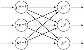
Diagonal state dependencies (as in Fig. 1) with t - 1 ≤ s < t (acc. to Def. 1) are often due to syntactic constraints on (D)BNs and stand in conflict with an actual causality. Such dependencies exist causally at s = t, but create directed cycles. While conflicting with causality, further, dependencies on "sibling" states of one time slice are spread over the past. This means, indirect causes among siblings are not anticipated, or rather, that chain reactions are not covered.

Example 2.1 (Regulatory Compliance). In a company deliberately placed false information, e.g., faked payment sums for bribe money, might divulge throughout a company until every employee believes (unknowingly) in a lie. We therefore model a probabilistic regulatory-compliance checking tool using a DBN to track and query possible violations of employees over time and to track back potential sources of deliberately placed false information. If one employee believes in false information, we do not say that such an employee is "corrupt", but say that he is credulous. Every employee, Claire, Don and Earl, say, is represented by one state in ⃗Xt . The probability P (Xt i ), encodes the belief in employee Xi being credulous xti or being integrous ¬xti at time t. We model B0, s.t., it models our prior belief in every employee being a source of false information, i.e., B0 is a BN containing all ⃗X0 as prior random variables; say P (c0 ) = 0.9, P (d0 ) = 0.6, P (e0 ) = 0.01. Being credulous is permanent, such that B→ describes all random variables Xt i depending on Xt-1 i with conditional probability P (xti |xt-1 i ) = 1.

An employee might influence another employee in his writings or, rather, in his information state. A credulous employee might therefore (undeliberately) influence his colleague such that the colleague also believes in false information, i.e., becomes credulous, too. Say, Claire influences Don, and if Claire is credulous, there is a probability of Don becoming credulous too. Further, if Don influences Earl, there is a probability that Claire influences Earl indirectly through Don. We can model this correctly as a dependency as C t → Dt → Et in B→. We assume an individual probability of 0.8 for an employee becoming credulous when being influenced by a credulous person and a noisy-or combination for every state.

However, we want to model that all employees can influence each other, and, to assure an acyclicity constraint, we must bend the influencing dependency to a consecutive timestep in B→ (as in Fig. 1). This is unavoidable, but is inaccurate from a world representation point of view, as indirect influences are now anticipated spuriously. Earl is now influenced by Claire through Don from a Claire of the penultimate time. This means, a time slice must be infinitesimal small, e.g. secondly, to anticipate all indirect influences, and cannot be chosen freely to an intended use case, e.g. daily.

In our example, we now can make observations, e.g., from unheralded compliance checkups and trace a potential diffusion of false information throughout our company over time. Still, we cannot actually model an accurate representation of a world, because we have to use a modeled dimension (time) for assuring syntactic constraints of (in)dependencies.

Classically a conditional independency in a Bayesian network is represented by the lack of an arc between two nodes. Another kind of independencies in Bayesian networks, called context-specific independencies (CSIs), has been studied by [Boutilier et al., 1996] & [Ngo and Haddawy, 1997] and has mainly been used for more efficient inference in such networks. CSIs represent dependencies in a BN that are only present in specific contexts. We extend this idea by defining special activator random variables.

Definition 2 (Activator Random Variable). We define AXY to be an activator random variable which activates a dependency of random variable Y on X in a given context. Let dom(AXY ) = {true, false} (extensions to non-boolean domains are straightforward). We define the deactivation criterion from a functional perspective towards the CPT as

where ∗ represents a wildcard and ⃗z further dependencies.

The activation criterion describes a situation where Y becomes dependent on X, i.e., the CPT entry for y is not uniquely identified by just aXY and ⃗z, hence

Example 2.2 (Activator). Claire does not constantly influence Don, but only if Claire sends a letter to Don. We can observe possible exchanges from used envelopes (possibly found in the trash bin). On such envelopes, we find multiple transfers from a coarse time interval in an imprecise or inaccurate order. For example, a transfer from Don to Earl and one from Claire to Don might include a transitive influence of Claire on Earl at the same time. A document transfer at time t, denoted M tCD , is then an activator for an influence of Claire C t on Don Dt . Likewise, if we can neglect this document transfer, i.e. observe ¬mtCD , Don becomes independent of Claire at time t.

The example shows that sometimes dependencies are modeled in B→ that are not always needed.

3 Activator Dynamic Bayesian Networks

We extend Bayesian networks such that, besides state variables, we have activators purely acting as necessary conditions for context-specific (in)dependencies.

Notation 3.1 (Activator Matrices). Let As t describe the matrix of all activator random variables between time-slice s and t, s.t.,

Let ⃗As t i denote the i th column of As t and let ⃗As t denote the corresponding column vector of all entries of As t , s.t.

Definition 3 (Activator Dynamic Bayesian Network (ADBN)). An ADBN fragment template B′→ consists of dependencies between states Xs i andXt j , t-1 ≤ s ≤ t (Markov1) and matrices As t of activators. Let As t ij be the activator random variable influencing Xt j regarding a dependency on Xs i , such that Xt j 's local CPT follows Eq. 2 and Eq. 1. Every activator is assigned a prior probability. An ADBN is then syntactically defined by (B0, B′→) defining its semantic as a joint probability P( ⃗X0:tᵀ , ⃗A01:ttᵀ ). ▲

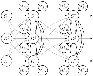
Still, t - 1 ≤ s < t is necessary to absolutely assure an acyclicity constraint when modeling ADBNs. Under the condition t - 1 ≤ s ≤ t, possibly directed cycles are created. For our work we only consider the problematic t-1 ≤ s ≤ t case, only containing in-time-slice dependencies (as in Fig. 2). For brevity, we write At for Att excluding Att kk , and, correspondingly, At and Atij .

The constraint t - 1 ≤ s < t for assuring acyclicity even in complete digraphs limits a causal reasoning process to direct dependencies between states.

Proposition 1 (Diagonal (A)DBN Restrictions). A classic, "diagonal" (as in Fig. 2) (A)DBN of type t - 1 ≤ s < t is restricted in its usage to special observation sets. Indirect influences are spread over multiple timesteps and possible indirect influences inside one timestep cannot be considered. This enforces a) an infinitesimal resolution of observations, where indirect effects do not need to be anticipated or b) restricts a DBN to observations where indirect influences strictly do not occur. This implies, not a single two activators At∗i and Ati∗ are allowed to be probably active, i.e. the set of probably active activators must form a bipartite digraph with uniformly directed edges. Further, only up to n2 /4 activators are allowed to be probably active per timestep, and all other activators must be (i) observed to be (ii) deactive. If, in a diagonal DBN, observations can neither hold a) or b), observation- and query-(de)serializations would be needed, and n - 2 spurious "time"-slices would need to be inserted between t - 1 and t. In our opinion, this degrades a BN to a reasoning tool. ▲

We show, by using a modified acyclicity constraint, that in ADBNs (Fig. 2) we can correctly anticipate indirect influences by modeling dependencies causally correctly.

Example 3.1 (Example continued). By extending our credulousness representing DBN with document transfer activators we obtain an ADBN with activators ⃗At = (M tCD ,M tDC ,M tDE ,M tED ,M tCE ,M tEC ) and states ⃗Xt = (C t ,Dt ,Et ). For every t we assume a prior probability for any transfer of P(mtij ) = 0.5. Still, we have to assume that every employee can influence every other, i.e., send him a document. To cover chain reactions of multiple transfers, we would then need syntactically forbidden cyclic dependencies.

The following Thm. 1 states that by using an ADBN it is indeed possible to move an acyclicity constraint from a design phase to an operations phase while maintaining a solid mathematical basis in accordance with Bayesian network semantics. This means, if the only possible mails are from Claire to Don to Earl, we could have modeled all influences correctly in one timestep during design of the DBN. Unfortunately, we do not know possible observations during design and such acyclic mail exchanges may differ in every time step.

Notation 3.2 (Vector Operands). Let fΓ( ⃗X, Y ) be the product of applied operands f to every row {1 ≤ i ≤ rank( ⃗X)}\Γ, i.e., we iterate over every row of ⃗X without rows in the set Γ and apply f to this row's elements. Scalars Y are used in every row, i.e.,

Notation 3.3 (Lexicographic Order). Let ≺ be a lexicographic term order, such that Xt-1 ∗ ≺ Xt∗ , Xt i ≺ Xt i+1 , and At-1 ∗∗ ≺ At∗∗ , Ati∗ ≺ At(i+1)∗ , Atij ≺ Ati(j+1) , and At∗∗ ≺Xt∗ , Xt-1 ∗ ≺ At∗∗ .

Theorem 1 (Bayesian Network Soundness). For every set of combinations of ⃗A1:t an ADBN (as in Fig. 2) corresponds to a Bayesian network, if, for all t, ⃗At satisfies the new acyclicity constraint:

with a function A (i, j)t that is defined as

Following the lexicographic order, the joint probability (JP) P( ⃗X0:tᵀ , ⃗A1:tᵀ ) of an ADBN is specified by,

written for brevity using Not. 3.2 as

As expected, the JP can be defined recursively:

Informally, Eq. 3 states that a deactive activator must break open dependency cycles, i.e., the set of possibly active activators forms a directed acyclic graph (DAG).

Proof of Theorem 1. We show that for every set of combinations of ⃗A1:t the joint probability stated in Thm. 1 is unique and well-defined, iff for all t the set of ⃗At obeys Eq. 3. We show this by reversing conditional independency assumptions in the semantic JP and find the unique topological order of our syntactical graph structure.

We begin with B0, which can be written as

with

Consecutively, we roll up the joint distribution according to Bayes' chain rule. Considering an extreme case of a set of activators corresponding to Eq. 3, it is straightforward that under Eq. 3 there must always ∃X1E1 : ∀iA1i(E1) = ¬a1i(E1) , such that due to Eq. 1, the set of activators and previous states uniquely identify the CPT entry and X1E1 becomes independent of all other ⃗X1 , such that the JP can be written as

By reversing X1E1 's conditional independency we can write

we can combine P( ⃗X0ᵀ ) with P( ⃗A1ᵀ ) to P( ⃗A1ᵀ , ⃗X0ᵀ ), s.t. the first eliminated state variable X1E1 can be combined to

Consecutively, there ∃X1E2 : ∀{i\E1}A1i(E2) = ¬a1i(E2) ,

for which we can reverse the conditional independency again and obtain

which, according to Bayes' chain rule, can be written as

Consecutively repeating this process for every further XEi, where the ith elimination variable is maximally dependent on the previous (i - 1) elimination variables, we, henceforth, approach the elimination of X1En , which is dependent on up to every other ⃗X1 , which are in fact all eliminated variables up to now, s.t.

for which we can reverse the conditional independency again and combine the JP finally to

Indeed, we already obtained a partial topological order > of X1En > X1E(n-1) > . . . > X1E1 > ⃗A1ᵀ > ⃗X0ᵀ . Following this procedure for the remaining t, we finally obtain

With a final reverse conditional independency assumption,

we obtain a complete topological order and a unique JP of

We have shown that the claimed JP of Th. 1 in fact is a unique and well-defined JP defining a topological order of a corresponding Bayesian network.

Informally speaking, this proof shows that in an ADBN an acyclicity constraint can be postponed to an operation phase while assuring soundness with BNs. This means, a BN can actually be a cyclic graph, if it is used correctly.

Proposition 2 (Completeness). An ADBN can model any JP. We have shown that in an ADBN all random variables of t can be dependent on each other, as long as during operations only certain combinations of activators are used. This means, that any form of in-time-slice structure can be modeled through adequate specifications of ⃗At . Straightforwardly, this can, if causally needed, be extended to further "diagonal" dependencies between states of consecutive time slices, including activator random variables for those dependencies. Obviously, this does not create cyclic dependencies and thus satisfies Eq. 3, i.e., is an ADBN. Such an ADBN would contain all possible dependencies between states and leave the option to (de)activate them, meaning, represents the most general form of an Markov-1 ADBN template including all possible Markov-1 DBN structures. Noteworthy, we can directly embed [Pearl, 2009]'s do-calculus here using activators. ▲

4 Operations

Based on Thm. 1 marginalization is well-defined and filtering, smoothing and prediction (according to the meaning of [Murphy, 2002]) can be derived from the joint distribution. We derive those operations while carefully handling novel in-time-slice dependencies and activator random variables.

Notation 4.1 (Notation for Observations). Let ⃗Z t ⊆ ⃗Xt be a set of observed and ⃗ ζ t = ⃗Xt\⃗Z t be the corresponding set of not-observed state variables. Let Bt ⊆ At be a set of observed activators and ⃗Bt ⊆ ⃗At be the corresponding column vector representation. Likewise, let ⃗ βt = ⃗At\⃗Bt be the column vector of all not-observed activators. We write ⃗z t for ⃗Z t = ⃗z and⃗b t for ⃗Bt =⃗b.

Every query contradicting with observations, i.e., ⃗xt contradicts ⃗z t , is defined to be of probability 0. Further, every observation in ⃗z t uniquely defines its corresponding random variable in ⃗Xt .

4.1 Filtering

We calculate the complete conditional joint probability P( ⃗X0:tᵀ , ⃗A1:tᵀ |⃗z 0:tᵀ ,⃗b 1:tᵀ ) at every timestep, from which every desired filtering operation can be marginalized out. With a normalization factor α, filtering is generally defined from the JP as

where all values of variables ⃗Xt , ⃗At are defined by the query and variables ⃗X0:t-1 , ⃗A1:t-1 are defined by either observations in the sets ⃗z 0:t-1 ,⃗b 1:t-1 or through summation over unobserved variables in ⃗ ζ 0:t-1 , ⃗ β1:t-1 .

Definition 4 (Filtering). Using the recursive definition of the joint probability in Eq. 4, filtering is efficiently defined as

ADBN filtering from t - 1 to t has time and space complexity O(1). Every incremental ADBN filtering is n-times faster than performing it in a serialized fashion having further O(t) space complexity for storing all orders. Further effort would be needed for generating such a serialized order.

Example 4.1 (Filtering). With Thm. 1 we can actually model cyclic dependencies as desired in Ex. 3.1 and build an ADBN for our example as shown in Fig. 2.

Say, Don and Earl did pass an initial checkup, but Claire did not. At t = 1, we observe a document transfer from Claire to Don, we are unsure about one from Don to Earl, but can neglect all other transfers. As Claire is credulous, we expect her to influence Earl slightly through Don, expressible in the filtering operation P (E1 |⃗z 0:1ᵀ ,⃗b 1ᵀ ), with ⃗z 0:1 = (c0 , ¬d0 , ¬e0 )ᵀ , and ⃗b 1 = (m1CD , ¬m1DC , ¬m1ED , ¬m1CE , ¬m1EC )ᵀ .

A diagonal DBN cannot anticipate the indirect influence, because t1-Earl is influenced by a t0-Don that has not received a document from Claire. This means our belief in Earl remains at 0 due to our initial observation of ¬e0 , i.e. P ′ (E1 |⃗z 0:1ᵀ ,⃗b 1ᵀ ) = 〈0, 1〉. As ⃗b 1 fulfills Eq. 3 we correctly obtain P(E1 |⃗z 0:1ᵀ ,⃗b 1ᵀ ) = 〈0.32, 0.68〉 using an ADBN, i.e. we anticipate that Earl is influenced by Claire through Don.

To achieve the same result in a diagonal DBN, we need observations at a finer time scale, where all indirect influences are serialized, e.g., we must first observe m1CD , anticipated in the filtering operation P ′ (E1 |⃗z 0:1ᵀ ,⃗b 1ᵀ ) and then insert a "correcting" "time"-slice t = 1.1, where we anticipate the possibilities of M 1DE in another operation P ′ (E1.1 |⃗z 0:1.1ᵀ ,⃗b 1:1.1ᵀ ). To achieve the result of one ADBN operation, we need n - 1 "diagonal"-operations.

Prediction is a filtering operationwith an empty observation set. However, as a minimal set of observations is needed to remove cycles, plain prediction is not possible in our syntax. However, by splitting a prediction-observation-set into two subsets, e.g. first the lower triangle and second the upper triangle of At+1 is observed to be deactive, prediction becomes possible. While this does not cover all possible chain reactions, it then covers significantly more than a classic DBN could cover (none), as previously discussed in Sec. 3 and Prop. 1.

4.2 Smoothing

Similar to the filtering operation, the general smoothing operation P( ⃗Xkᵀ , ⃗Akᵀ |⃗z 0:tᵀ ,⃗b 1:tᵀ ), k < t can be derived from the joint probability as

in which we find a previous (stored) filtering operation, known as a forward message, and a new latter term commonly known in smoothing operations. Using an adequate recursive definition for the latter term, we obtain an efficient calculation method using a "backward message." The commonly known "sensor model" is, due to in-time-slice dependencies, included in the forward, as well as backward message.

Definition 5 (Smoothing). Smoothing at timestep k considering all evidences up to t is defined as

The last term corresponds to the backward message and was calculated in the previous (i.e., previously calculated, but temporally consecutive) smoothing operation. ▲

Performing smoothing over all k < t has O(t2 ) time and constant space complexity or, by storing filtering operations, O(t) time and space complexity. Compared to a serialized version, without actually serializing, n2 -times faster or ntimes faster and smaller.

Example 4.2 (Explaining away). Continuing Ex. 4.1 this example demonstrates that smoothing handles explaining away over multiple timesteps and respects indirect causes. Say, only Don underwent a successful compliance check at time t = 0, i.e., ⃗z 0 = (¬d0 ). For t = 1 we found the same document transfer as previously, and for t = 2, a Sunday, we can neglect all, i.e., ⃗b 2 = ∅. On that Sunday also irregularities in Earl's documents were found, i.e., ⃗z 2 = (e2 ).

If we perform the smoothing operation for Claire's initial belief state without considering evidence from t = 2, we end up with our prior belief of P(C 0 |⃗z 0:1ᵀ ,⃗b 1ᵀ ) = 〈0.5, 0.5〉, as we have gained no new information. However, with observations from t = 2, we need to consider an indirect influence by Claire onto Earl and our belief in her rises to P (C0 |⃗z 0:2ᵀ ,⃗b 1:2ᵀ ) ≈ 〈0.532, 0.468〉.

The slow increase is due to our high prior belief in Earl manipulating documents of P(e0 ) = 0.7 and it is more likely that Earl has been manipulating documents ever since. If, say, Earl can be relieved from initial incriminations, i.e., ¬e0 , the only explanation for this situation is an indirect cause of Claire being credulous, which is correctly handled as P (c1 , m1DE |⃗z 0:2ᵀ ,⃗b 1:2ᵀ ) = 1. We can update our initial prior beliefs using smoothing and find that P (d0 ) = P (e0 ) = 0 but P(c0 ) = 1. We can now say for sure, Claire is corrupt.

In a classic diagonal (A)DBN the last example would have been unexplainable, as indirect influences of t1 (causally) would first be anticipated a step later at t2 (for n=3). The detailed explanation is confusing, because it is not causal: at t2, the time of incriminating evidence for Earl, we know that Earl is only influenced by himself, i.e. only t1-Earl can be the source of his credulousness. At t1, Earl only receives a document from integrous t0-Don (observation). This is where the problem lies, t0-Claire should have influenced t0-Don by now, but t0-Claire influences t1-Don with her message m1CD . I.e. Earl cannot become credulous and the observation e2 remains unexplainable. Mathematically we obtain P(e0 |⃗z 0:2ᵀ ,⃗b 1:2ᵀ ) = 0 because all terms in this calculation involve either the CPT entry P (e2 |¬m2∗E , C1 , D1 , ¬e1 ) = 0 or P (e1 |M 1DE , ¬m1CE , C0 , ¬d0 , ¬e0 ) = 0 (Underlined CPT attributes uniquely identify these entries to be 0). By definition, we obtain P(¬e2 | . . . , e2 , . . .) = 0, and, thus, we stand in conflict with the probability axioms of Kolmogorov.

5 Discussion

Using an ADBN has the benefit of anticipating indirect causes in-time in an over-the-time evolving process. Still, it comes with a cost of introduced activators, which need to be defined and enforce minimal observation sets of activators (Eq. 3: any acyclic constellation of probably active activators is allowed). However, we came from a point of view where activators existed and Prop. 1 shows that classic DBNs are significantly more restricted (the number of uniformly directed bipartite graphs with n vertices is far smaller than the number of possible DAGs). The need to anticipate indirect influences originated from coarse observation timesteps, where indirect influences must be anticipated to explain made observations. Where we motivated coarse timesteps from an unavailability of finer observations, the choice of coarser timesteps is also motivated by computational feasibility. Not being bound to the finest available observation granularity relaxes the rate of needed time-updates and is also discussed by [Pfeffer and Tai, 2005] in the form of Asynchronous DBNs using [Nodelman et al., 2002]'s CTBNs. Still, Asynchronous DBNs and CTBNs run into the same problem given in Prop. 1 of anticipating indirect influences during one timestep.

We have discussed the complexity of operations over time and have shown that in an ADBN we obtain the same, and even simpler, complexities as in classic DBNs. However, like in any other DBN, the dimension complexity in terms of nodes of one operation remains computationally intractable and demands approximate inference techniques, which can greatly benefit from context specific independencies, as shown by [Boutilier et al., 1996].

Notwithstanding, it is possible that Eq. 3 does not hold in a particular situation. Still, we now have a direct indicator for potentially spurious results. In this particular situation a mitigation is needed, but is beyond the scope of this paper. Such a mitigation would be, for example, to move small subsets of activators to a neighboring timestep or enforcing observations of more deactive activators.

6 Conclusion

We have shown that indirect causes in dynamic Bayesian networks cause conflicts in representing causality. These conflicts arose from using a modeled dimension for assuring syntactic requirements. By extending dynamic Bayesian networks with activator variables to ADBNs, we are able to move acyclicity constraints from a design phase to a later operation phase. Without the need of algorithm frameworks, degrading a Bayesian network to a reasoning process, we obtained a solid mathematical basis sound to Bayesian networks with a causally correct anticipation of indirect causes in dynamic Bayesian networks under much softer restrictions.

Future work is dedicated to further acyclicity constraints when considering properties of local CPDs, which even allow operations with cyclic activator sets and extensions to relational Bayesian networks [Jaeger, 1997].