
Algorithm Portfolios Based on Cost-Sensitive Hierarchical Clustering
Proceedings of the Twenty-Third International Joint Conference on Artificial Intelligence. Pages 608-613.
© 2013 International Joint Conferences on Artificial Intelligence
Abstract
Different solution approaches for combinatorial problems often exhibit incomparable performance that depends on the concrete problem instance to be solved. Algorithm portfolios aim to combine the strengths of multiple algorithmic approaches by training a classifier that selects or schedules solvers dependent on the given instance. We devise a new classifier that selects solvers based on a cost-sensitive hierarchical clustering model. Experimental results on SAT and MaxSAT show that the new method outperforms the most effective portfolio builders to date.
- [Amadini et al., 2013] Roberto Amadini, Maurizio Gab- brielli, and Jacopo Mauro. An empirical evaluation of portfolios approaches for solving csps. In CPAIOR-2013, 2013.
- [Elkan, 2001] Charles Elkan. The foundations of cost- sensitive learning. In IJCAI-01, pages 973-978, 2001.
- [Geibel and Wysotzki, 2004] Peter Geibel and Fritz Wysotzki. Learning perceptrons and piecewise lin- ear classifiers sensitive to example dependent costs. Appl. Intell., 21(1):45-56, 2004.
- [Gomes and Selman, 2001] C.P. Gomes and B. Selman. Al- gorithm portfolios. Artificial Intelligence Journal, 126(1- 2):43-62, 2001.
- [Guyon and Elisseeff, 2003] Isabelle Guyon and André Elis- seeff. An introduction to variable and feature selection. J. Mach. Learn. Res., 3:1157-1182, 2003.
- [Kadioglu et al., 2010] S. Kadioglu, Y. Malitsky, M. Sell- mann, and K. Tierney. Isac -instance-specific algorithm configuration. Proc. of the 19th European Conference on Artificial Intelligence (ECAI), pages 751-756, 2010.
- [Kadioglu et al., 2011] S. Kadioglu, Y. Malitsky, A. Sabhar- wal, H. Samulowitz, and M. Sellmann. Algorithm selec- tion and scheduling. CP, 2011.
- [Klinkenberg and Rüping, 2003] Ralf Klinkenberg and Ste- fan Rüping. Concept drift and the importance of example. In Text Mining, pages 55-78, 2003.
- [Lenarcik and Piasta, 1998] Andrzej Lenarcik and Zdzislaw Piasta. Rough classifiers sensitive to costs varying from object to object. In Rough Sets and Current Trends in Computing, pages 222-230, 1998.
- [Malitsky, 2013] Yuri Malitsky. Algorithm portfolio bench- mark set, 2013. http://4c.ucc.ie/ ∼ ymalitsky/algorithm portfolio benchmark set.html. Link
- [O'Mahony et al., 2008] E. O'Mahony, E. Hebrard, A. Hol- land, C. Nugent, and B. O'Sullivan. Using case-based reasoning in an algorithm portfolio for constraint solving. Irish Conference on Artificial Intelligence and Cognitive Science, 2008.
- [Silverthorn and Miikkulainen, 2010] B. Silverthorn and R. Miikkulainen. Latent class models for algorithm portfolio methods. AAAI, 2010.
- [Stern et al., 2010] D. Stern, H. Samulowitz, R. Herbrich, T. Graepel, L. Pulina, and A. Tacchella. Collaborative ex- pert portfolio management. AAAI, 2010.
- [Streeter and Smith, 2007] M. Streeter and S.F. Smith. Using decision procedures efficiently for optimization. ICAPS, pages 312-319, 2007.
- [Ting, 2002] K. M. Ting. An instance-weighting method to induce cost-sensitive trees. IEEE Trans. on Knowl. and Data Eng., 14(3):659-665, 2002.
- [Wysotzki and Geibel, 2009] Fritz Wysotzki and Peter Geibel. A new information measure based on example- dependent misclassification costs and its application in decision tree learning. Adv. Artificial Intellegence, 2009.
- [Xu et al., 2008] L. Xu, F. Hutter, H.H. Hoos, and K. Leyton- Brown. Satzilla: Portfolio-based algorithm selection for sat. JAIR, 32(1):565-606, 2008.
- [Xu et al., 2012a] L. Xu, F. Hutter, J. Shen, H.H. Hoos, and K. Leyton-Brown. Satzilla2012: Improved algo- rithm selection based on cost-sensitive classification mod- els. solver description, 2012. SAT Challenge 2012.
- [Xu et al., 2012b] Lin Xu, Frank Hutter, Holger Hoos, and Kevin Leyton-Brown. Evaluating component solver con- tributions to portfolio-based algorithm selectors. In SAT- 2012, pages 228-241, 2012.
- [Zadrozny et al., 2003] Bianca Zadrozny, John Langford, and Naoki Abe. Cost-sensitive learning by cost- proportionate example weighting. In 3rd Intl. Conf. on Data Mining, pages 435-442, 2003.
References were extracted automatically from the PDF and may contain errors.
Full text extracted automatically from the PDF; figures, tables and equations may differ. The PDF is the version of record.
1 Introduction
Algorithm portfolios are an essential tool for boosting problem solving performance. In essence, the idea of algorithm portfolios is to select one or schedule several solvers out of a pool of algorithms based on the problem instance that is to be solved. This technology has proven key for providing state-of-the-art performance in satisfiability (SAT), quantified Boolean formulae (QBFs), and constraint programming (CP) as exemplified by the performance of portfolios in the respective solver competitions.
1.1 RelatedWork on AlgorithmPortfolios
Algorithm portfolios, at least in their most recent advent, were pioneered by Gomes and Selman [2001] and Xu et al. [2008]. The first really prominent instance of a solver portfolio was SATzilla 2007, a SAT solver portfolio. It was based on a linear regression model to predict log runtime for each solver. For a while, the trend was towards more sophisticated machine learning models, such as a hidden-class portfolio generator [Silverthorn and Miikkulainen, 2010] or collaborative expert portfolio management [Stern et al., 2010]. In parallel, the idea to schedule solvers, meaning, to run a selection of solvers for some designated time, was introduced by Streeter and Smith [2007] and O'Mahony et al. [2008].
Based on these methods, Kadioglu et al. [2011] introduced the idea of scheduling solvers while still picking one longrunning solver. The notable feature of this portfolio, named 3S, was that it used a low-bias (the authors call it "non-model based") machine learning technique for selecting the long
Ashish Sabharwal, Horst Samulowitz, Meinolf Sellmann
IBM Watson Research Center
Yorktown Heights, NY 10598, USA
{ashish.sabharwal,samulowitz,meinolf}@us.ibm.com
running solver. Namely, the latter is conducted by means of a k-nearest neighbor approach which proved very effective for SAT. The 2011 and 2012 incarnations of SATzilla [Xu et al., 2012a; 2012b] followed this trend and introduced a cost-sensitive, low-bias classification model approach based on random forests and voting. A recent comparison of the SATzilla-2012 and the 3S portfolio building approaches was conducted by Amadini et al. [2013] for building a portfolio of CP solvers which revealed a statistical tie between both methods for this benchmark, whereby 3S appears to be performing marginally better.
1.2 Motivation and Scope
The motivation of this work is to provide a portfolio builder that works efficiently across a wide range of problem domains. For SAT and for CP we have fairly well-established feature sets that can be used to characterize a given problem instance and predict which solver(s) will be most effective at solving it quickly. However, we strongly believe that algorithm portfolios could be equally effective in boosting solver performance in other domains, such as MaxSAT or global continuous optimization or mixed-integer programming (MIP) where no good feature sets are readily available.
We expect that the SATzilla-2012 methodology will generalize to other domains better than 3S as each feature that has little predictive power regarding which solver is better suited for solving a problem deteriorates k-nearest neighbor-based 3S performance. While there are ways to handle this (e.g., feature selection [Guyon and Elisseeff, 2003]), it is at the very least tedious for the non-expert to have to select the right features. Moreover, even when using scaling techniques, k-nearest neighbor cannot give different weight to features in different parts of the feature space. SATzilla-2012 on the other hand can easily accommodate features which are not helpful and use features only in those areas of the search space where they actually help us differentiate between solvers.
On the other hand, 3S's scheduler is based on traditional optimization MIP technology while SATzilla-2012 uses a heuristics-based presolver schedule. Surprisingly, we found that training this presolver takes a significant amount of time in SATzilla-2012. Furthermore, SATzilla-2012 trains one random forest for each pair of solvers. This creates a computational bottleneck as the training time obviously squares when the number of solvers doubles. One goal of this paper is to perform cost-sensitive multi-class classification directly and not by means of binary classification in order to alleviate this computational burden.
We propose a new portfolio builder that combines 3S's static scheduler with a new algorithm selector based on costsensitive hierarchical clustering (CSHC) which creates a multiclass classification model, runs orders of magnitude faster than SATzilla-2012, and is less sensitive to poor feature sets than 3S. We describe the method in detail and provide extensive empirical results comparing CSHC with SATzilla-2012 and 3S on various benchmark sets for portfolio generators.
2 Toward ANewAlgorithmPortfolio Builder
Clustering is a standard technique in unsupervised learning, equally fundamental and simple as k-nearest-neighbor classification in supervised learning. The two methods bear methodological similarities as well. The result of k-nearest neighbor learning is the labeling of compact areas of the feature space by one class, just as clustering groups of instances into compact clusters. In fact, the k-nearest-neighbor in 3Swas inspired by cluster-based instance-specific algorithm configuration shown by Kadioglu et al. [2010].
While clustering is certainly appealing, it makes sense to center clusters at the test instance that needs to be solved. That is exactly what the k-NN approach does. Moreover, traditional clustering is unsupervised. For the purpose of algorithm portfolios, we would like to group training instances in such a way that they can agree on the class they should be labeled with. For us that means that training instances in the same cluster should preferably not disagree violently on which solver solves themmost efficiently (or at all, in case of timeouts). Finally, while clustering is traditionally based on some metric of distance, to accommodate poor feature sets we need a clustering method that allows us to select when or under what circumstances we use the dimensions that features provide are used for determining what goes into the same cluster.
2.1 Cost-Sensitive Hierarchical Clustering
We propose a learning method which we named cost-sensitive hierarchical clustering (CSHC). High-level, the method proceeds as follows. First, all instances are in the same cluster. Now, for each cluster in the current set of clusters, we test whether a given minimum number of instances is still present in that cluster (we typically set this required minimum to ten instances). If not, we remove the cluster from consideration for further partitioning. Otherwise we split the cluster in such a way that the instances within each of the two clusters maximally agree on the class they should be labeled with.
We will investigate a variant where we add another phase, where we consider merging clusters again for which the split resulted in diminishing cross-validation performance.
At run-time, we compute the given instance's feature vector and determine which cluster it belongs to. Then, we employ the solver that performs best on the training instances in this cluster.
Cost-Sensitive Learning Problem
More formally, we consider the following (incomplete) classification problem. Given are a set of classes C and a set of training instances T , each associated with a feature vector f ∈ IRF . Moreover, we are provided with a cost-vector that associates each instance i ∈ T with a cost mi,c ≥ 0 which represents the cost of (mis-)classifying instance i by class c ∈ C. The task is to infer a classification algorithm which will assign a class to new instances such that their associated misclassification cost is minimized. We label this classification problem incomplete as we obviously do not know what the misclassification costs for the given instance are or how these can be inferred from the misclassification costs that we observe for the training instances.
It is worth noting that the problem considered is similar yet fundamentally different from semi-supervised problems considered in machine learning. In particular, Elkan [2001] considered the problem where the misclassification costs are determined by a given |C| × |C| matrix which assigns a misclassification cost to each pair of classes, where the first is the preferred class of the instance, and the second is the class we label it with. Obviously, when building an algorithm portfolio, there does not exist and, in any case, we would not have access to such a class-misclassification matrix.
It is interesting to note that the model-based portfolio approaches [Xu et al., 2008; Silverthorn and Miikkulainen, 2010] essentially aim to predict the misclassification costs for a given instance. One advancement was the realization that better predictions are obtained when we focus on predicting a preferred class without taking the detour of forecasting the misclassification costs for each class for the given instance [O'Mahony et al., 2008; Kadioglu et al., 2011; Xu et al., 2012b].
There exist many other cost-sensitive learning methods (see for example [Lenarcik and Piasta, 1998; Ting, 2002; Zadrozny et al., 2003; Klinkenberg and R¨uping, 2003; Geibel and Wysotzki, 2004; Wysotzki and Geibel, 2009]). It is beyond the scope of this paper to give a comprehensive overview. However, the only cost-sensitive multiclassification approaches for the cost-model that applies to portfolios that we are aware of are the ones employed by 3Sand SATzilla-2012, whereby the latter is based on a series of binary classifications.
Approach
During CSHC's learning phase we maintain a set of clusters, starting with all training instances in one cluster. In each iteration, we remove one cluster from the current set. If it is too small, we do not partition it further. Otherwise, we partition the cluster in two parts by running a hyperplane through the feature space so that instances fall on either side of the plane.
When labeling an instance i with class C we incur the cost m(i,C). The total (mis)classification cost when labeling a subcluster with a specific class is the sum of all costs for all instances in that cluster. The cost of a binary split is the cost of labeling each subcluster with a class that gives the lowest cost. We select a hyperplane to split the cluster so that the cost of the binary split is minimized. If none of the sub-clusters are empty, we add both to the current set of clusters.
In a potentially following phase, we consider undoing some cluster splits based on the cross-validation performance that we would achieve by labeling the whole cluster with one class, compared to the cross-validation performance when doing the same for the two sub-clusters. If the performance of the split is not better, we undo the partition.
At runtime, for the first 10% of available time, the portfolio executes the same static schedule as 3S. If this does not result in a solution, we use the hyperplanes used for splitting the base set to determine which cluster the test instance belongs to, and we try solving it with the solver that has the overall best performance on all training instances in that cluster.
Decision Trees
As we will discuss shortly, in practice we will consider axisparallel hyperplanes to obtain a tractable training method. This means that the clustering approach could very well also be viewed as a decision tree approach where the ground set of training instances is repeatedly partitioned by branching on individual features. The main difference to existing costsensitive desision tree methods is the way how we compute the cost of a split. Instead of considering entropy or costsensitive entropy, we favor splits where, in both parts, the instances can agree on a consensus label that may not be perfect for any one instance but that incurs minor costs for all.
2.2 Bagging, Maximum-Margin Hyperplanes, Feature Augmentation
In this section, we discuss several alternative techniques that we considered adding to the basic CSHC methodology. Later we will test these empirically and quantify their effect on overall portfolio performance.
Bagging
The first technique we consider is bootstrap aggregating (bagging), a well-known technique in machine learning for improving the stability of classification and regression algorithms. In our case, we generate bootstrap samples to create training sets which are then clustered. That is, rather than creating just one clustering using all training instances, we create multiple clusterings based on subsets of the training set.
The obvious question arises how we should then combine the potentially conflicting classifications from different clusterings. We propose four different ways on how this information can be combined:
- PAR-10 Aggregation: Collect, for each clustering, the respective training instances in each cluster that the test instance belongs to. We can assemble these instances into a set or a multi-set of instances. Then, to determine the solver the given instance should be solved with, we compute which solver has the best performance in terms of average runtime with timeouts penalized by a factor of 10 (PAR-10) on the set or multi-set of instances in the various different clusters the test instance belongs to.
- Winner Aggregation: Determine the best class for each cluster the test instance belongs to. Then we label the test instance with the class that was chosen most often.
- Rank Aggregation: Rank the classes in each cluster the test instance belongs to. Then, we choose the class that has the best average rank over all clusterings.
- SATzilla-style Aggregation: Recall that SATzilla-2012 builds a random forest for each pair of classes (which, in our case, correspond to solvers). Using the analogy of axis-parallel clustering and decision trees discussed above (the only difference being how we split), each random tree can be viewed as a "clustering" of training instances. In SATzilla-2012 the information from each "cluster" are aggregated by first aggregating over all trees, and then counting how many other solvers each solver is able to outperform. We can emulate this aggregation scheme by computing, for each ordered pair of solvers, for how many of our bagged clusterings the first solver outperforms the second. If this number is at least half, we say the first solver outperforms the second, otherwise we say the second outperforms the first. We then compute, for each solver, how many other solvers it outperforms. We choose the solver that outperforms the most other solvers.
Maximum-Margin Hyperplanes
Earlier, we said that we would compute a hyperplane to split the base instances such that the performance of the best solver on each side is maximized. This is, in general, a hard optimization problem. We consider two heuristics for computing such hyperplanes. The first is to consider feature-axisparallel hyperplanes only which renders the resulting optimization problem tractable. Using this method, our clustering approach can be viewed as a decision-tree procedure. In a second variant, we consider accepting the best split according to an axis-parallel hyperplane, but then tilt it so as to achieve a splitting hyperplane that achieves the same base partition with a maximum margin. We found that non-axis-parallel hyperplanes do not boost performance, yet increase the learning time considerably, which is why we do not pursue this avenue further in this paper.
Feature-Augmentation
One welcome advantage that CSHC shares with the SATzilla-2012 approach is the ability to accommodate features that have limited prediction potential. That is, we can add a bunch of new features or combinations of the existing features without fearing that performance would decline. We consider adding products and quotients of pairs of features to our feature set.
3 Analyzing the Components of CSHC
A priori it is not clear which of the variants of CSHC performs best. In this section, we therefore perform an experimental comparison of different versions of the cost-sensitive clustering approach we have proposed.
Typically, in the literature on algorithm portfolios we find that different papers consider different sets of features, differing sets of solvers, and differing train and test sets. Recently, Malitsky [2013] created an actual benchmark for algorithm portfolios that standardizes these choices. It allows us to compare different algorithm portfolio methods on a level playing field as the benchmark for a portfolio builder really consists of all, available features, the set of base solvers, as well as training and test sets.
All experiments in this section are based on the dataset provided by the UBC group 1 after SATzilla won the SAT Challenge 2012. The data is broken down into crafted, industrial, and random categories. Instances in each category were solved by the same 31 SAT solvers with a 1,200 second timeout. Malitsky [2013] removed all instances that cannot be solved by any solver within the allotted timeout and broke down each of the data sets into 10 parts suitable for cross-fold validation. Instances are characterized by the 125 features the UBC team proposed (option -base). For each of the three benchmark sets, we created five benchmarks with two, three, four, twelve, and all 31 solvers by removing solvers from the base set.
In the rest of this section, we evaluate the contribution of various components of CSHC to its performance and use the findings to tune basic choices in CSHC (how many clusterings to use, what aggregation mechanism to use, etc.). In Section 4 we then compare the resulting tuned CSHC with other portfolio solvers. To keep this latter comparison fair, we tune the components of CSHC on a different benchmark than the benchmarks we will use later to compare with other portfolio builders.
3.1 Number of Bootstrap Samples
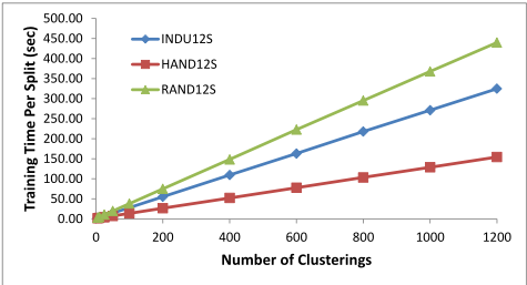
First, we investigate the impact of the number of clusterings on the robustness, stability, and scalability of CSHC. We ran CSHC with various numbers of bootstrap samples ranging from 5 to 1,200, whereby each sample contains 60% of all available training instances. We also tested various other percentages but that had little effect on the overall trend. The experiments were run on the benchmark data mentioned above and results reported are the averages over the 10 data splits used for cross-validation.
Figure 1 shows, for each number of clusterings on the horizontal axis, the average training time per split on the vertical axis. There is one curve each for the industrial, crafted, and random instance benchmarks. As expected, we see that the training time of CSHC scales linearly as the number of clusterings grows. Training never took more than 7 minutes 2 per split on this benchmark even with 1,200 clusterings. This is massively faster than SATzilla-2012 3 which, on these benchmark sets with 31 solvers, needs CPU-days to be trained.
1 http://www.cs.ubc.ca/labs/beta/Projects/SATzilla
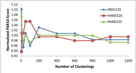
Figure 2 shows, again as a function of the number of clusterings, the normalized average PAR-10 score observed across the 10 splits. For each of the industrial, crafted, and random benchmark sets, the PAR-10 score plotted here is normalized by the average of the PAR-10 scores across all 10 splits. Note that, as the number of clusterings grows, this measure will eventually converge to 1, independent of the benchmark. We observe that CSHC is rather unstable for up to about 100 clusterings but begins to show reasonable stability after a few hundred clusterings.
While using more clusterings makes performance more robust, there is clearly a tradeoff with growing training time. For the rest of the experiments reported in this paper, we chose to use 800 clusterings which kept CSHC reasonably fast yet stable.
3.2 Aggregation
We discussed four different aggregation schemes earlier, PAR-10, winner, rank, and SATzilla-inspired aggregation. In Table 1 we present our numerical results when using these aggregators.
Our first observation from this data is that the SATzillainspired aggregation method is clearly inferior to all other techniques. Note that, while the method is inspired by SATzilla-2012, this does not mean that, within that portfolio builder, the aggregation method used is sub-optimal. First, SATzilla-2012 builds a different random forest for each pair of solvers. CSHC on the other hand builds just one set of clusterings which performs multi-class classification. The latter gives an advantage in terms of the time needed for learning. However, it may very well have an adverse effect on this aggregation method. Second, the way how we cluster the different bootstrap samples differs fundamentally from the costsensitive random-forests that SATzilla-2012 creates.
2 These experiments were conducted on a 4-core Intel Xeon 2.4 GHz machine with 24 GB RAM running Scientific Linux 6.1.
3 Downloaded from http://www.cs.ubc.ca/labs/beta/Projects/ SATzilla.
| SAT Family | PAR-10 | Winner | Rank | SATzilla |
|---|---|---|---|---|
| Crafted | 89.3 | 91.0 | 89.2 | 81.0 |
| Industrial | 96.4 | 96.6 | 97.2 | 87.2 |
| Random | 97.1 | 97.0 | 97.1 | 92.9 |
| SAT Family | #Solvers | PAR-10 | Winner | Rank |
|---|---|---|---|---|
| Industrial | 2 | 97.6 | 97.6 | 98.5 |
| 3 | 97.1 | 97.8 | 98.1 | |
| 4 | 97.6 | 97.8 | 97.8 | |
| 12 | 96.5 | 96.9 | 96.8 | |
| Crafted | 2 | 94.4 | 94.4 | 94.4 |
| 3 | 94.1 | 95.2 | 95.6 | |
| 4 | 92.9 | 92.9 | 93.3 | |
| 12 | 90.8 | 92.7 | 90.8 | |
| Random | 2 | 98.2 | 97.9 | 98.0 |
| 3 | 96.8 | 96.3 | 96.5 | |
| 4 | 96.4 | 96.5 | 96.3 | |
| 12 | 98.3 | 97.9 | 98.2 |
Between the remaining aggregators, there is no clear winner. We therefore created more benchmarks by selecting subsets of base-solvers. Table 2 shows the comparison between the remaining aggregators on these additional benchmarks. Overall, we find that the rank-based aggregation performs with good average performance while displaying the smallest variance in performance. It works second best on the crafted and random categories and, across the board, best on industrial instances.
3.3 Combination Features
As discussed earlier, unlike 3S, both CSHC and SATzilla-2012 can naturally accommodate more features and simply not use them if they are not helpful. Given k original features, we consider adding k′ randomly chosen pairwise products and quotients of these features to CSHC. If f2 = 0, the quotient f1/f2 is treated as 1 if f1 is also 0, and as a cutoff value of sign(f1) × 1036 otherwise.
| #Features | Industrial | Crafted | Random | |||
|---|---|---|---|---|---|---|
| added | PAR10 | TrTime | PAR10 | TrTime | PAR10 | TrTime |
| 0 | 494 | 3.8 | 1402 | 1.9 | 419 | 5.5 |
| 25 | 519 | 12.3 | 1423 | 6.8 | 419 | 24.9 |
| 50 | 507 | 23.5 | 1423 | 12.6 | 419 | 47.2 |
| 100 | 505 | 69.8 | 1316 | 30.3 | 397 | 119 |
| 150 | 493 | 135 | 1380 | 61.4 | 408 | 210 |
| 200 | 482 | 237 | 1426 | 123 | 420 | 300 |
| CSHC+Merging | CSHC | |||
|---|---|---|---|---|
| Benchmark | % | PAR-10 | % | PAR-10 |
| Industrial | 96.7 | 548 | 97.2 | 494 |
| Crafted | 88.9 | 1445 | 89.2 | 1423 |
| Random | 97.0 | 432 | 97.1 | 420 |
Table 3 shows the result of adding k′ = 0, 25, 50, 100, 150, and 200 such feature combinations. For each benchmark we report the resulting performance in terms of PAR-10 score averaged over the 10 splits, along with the average training time needed per split. We find that adding products and quotients does not lead to a substantial difference in the PAR-10 performance on this dataset, at least on the industrial instances. On crafted and random instances, using k′ = 100 results in a somewhat improved performance. However, the improvement is unstable across different benchmark categories and comes at the cost of 30 minutes to nearly 2 hours of training time per split, compared to under 6 minutes without these additional features. We therefore chose not to use such augmented features for the remainder of this empirical study.
3.4 Cross-Validation-BasedMerging of Clusters
When describing the CSHC approach we discussed the possibility of undoing cluster splits based on a cross-validation. We implemented this technique and compare it to the plain cost-sensitive hierarchical clustering we proposed.
We show our results in Table 4. Across the board we observe that the merging of split clusters actually diminishes performance. We tested a number of other techniques for undoing splits, such as merging if the performance of the split declines on the instances left out for training by the current bootstrap sample. However, all these techniques showed the same trend: The simpler technique of cost-sensitive hierarchical clustering without cluster-merging performs better. This observation matches the well-known fact that, when constructing decision forests, it is better not to prune the trees.
4 Comparison with SATzilla-2012 and 3S
There are two portfolios which excelled in the last two SAT Competition/Challenges. In 2011, 3S [Kadioglu et al., 2011] won the crafted and random categories. In 2012, SATzilla-2012 [Xu et al., 2012a] won the industrial and crafted categories.
[Amadini et al., 2013] compared the two approaches when building portfolios of constraint programming solvers. It was already noted there that SATzilla-2012 needed much more time for learning, especially as the number of solvers increases. In terms of test performance, Amadini et al. [2013]
Table 5: Performance comparison of 3S, SATzilla-2012, and CSHC on the MAXSAT benchmark. Shown are the average percent solved (timeout 1,800 seconds) and PAR-10.
| 3S | SATzilla-2012 | CSHC | 3S | SATzilla-2012 | CSHC | ||||||||
|---|---|---|---|---|---|---|---|---|---|---|---|---|---|
| MaxSat MS Crafted | % 99.4 | PAR-10 224 | % 99.3 | PAR-10 228 | % 99.4 | PAR-10 256 | Benchmark | % | PAR-10 | % | PAR-10 | % | PAR-10 |
| PMS Crafted | 95.3 | 1014 | 99.3 | 155 | 99.3 | 196 | Industrial | 88.0 | 6638 | 92.1 | 4444 | 93.1 | 4093 |
| PMS Indu | 96.4 | 728 | 98.1 | 412 | 98.3 | 391 | Crafted | 81.8 | 10453 | 89.5 | 5760 | 90.9 | 5169 |
| WPMS Crafted | 91.4 | 1683 | 95.0 | 948 | 97.0 | 609 | Random | 96.6 | 2004 | 98.2 | 1165 | 99.0 | 870 |
| WPMS Indu | 100 | 132 | 96.6 | 718 | 98.3 | 421 | |||||||
found that both builders result in almost the same performance, with a slight edge in favor of 3S which was not statistically significant. To the best of our knowledge, to date this is the only comparison of SATzilla-2012 and 3S on a level playing field where both builders use the same set of solvers, the same features, and the the same train/test splits.
4.1 MaxSAT
Using Malitsky's portfolio benchmark [Malitsky, 2013], we compare CSHC with 3S and SATzilla-2012. In Table 5 we compare CSHC with 3S and SATzilla-2012 on various MaxSAT benchmarks. All builders use the same set of base solvers and the same features that are provided for each instance. The numbers represent the average test performance over the same ten cross-validation splits that are part of the benchmark.
The benchmark consists of instances gathered from the various categories of the 2012 MaxSAT Evaluation. There are five benchmarks in total: crafted unweighted MaxSAT (MS), crafted and industrial partial MaxSAT (PMS), and crafted and industrial weighted partial MaxSAT (WPMS). These instances were run with a 1,800 second timeout with 10 to 14 MaxSAT solvers, depending on the benchmark. We use the ten cross-validation splits provided by [Malitsky, 2013].
For the features, the MaxSAT instance was converted into an equivalent instance where all the soft clauses are unit. This is achieved by reifying the soft clauses. Finally, the computation of the features is performed using the SATzilla featurecode on the hard clauses of the MaxSAT formula.
We observe that 3S's performance is rather erratic. At times it works really well, other times it works significantly worse than SATzilla-2012 and CSHC. It performs equally well as CSHC on crafted MaxSAT benchmarks, and it clearly outshines all other methods on weighted partial MaxSAT Industrial. On the other hand, it works much worse on all remaining benchmarks.
Comparing SATzilla-2012 and CSHC, we find that the latter performs on par on crafted partial MaxSAT and better on all other benchmarks. Especially on the two weighted MaxSAT benchmarks CSHC works notably better than SATzilla-2012.
4.2 SAT
Next we use the benchmark based on data from the SATzilla-2012 webpage. This data utilizes the dataset provided by the UBC group coupled with their SATzilla portfolio Matlab code. 4 The data is broken down into crafted, industrial, and random categories. Instances in each category were taken from the 2012 SAT Challenge and run on the solvers at that competition (15 for Crafted, 18 for Industrial, and 9 for Random). Timeout is 5,000 seconds. [Malitsky, 2013] again removed all instances that could not be solved by any solver within the allotted timeout and provided ten standardized cross-validation splits.
Consider Table 6. We observe the same trend as we had noted on the MaxSAT benchmarks. 3S behaves erratically: On the random category it performs almost as good as SATzilla-2012 and CSHC, but on the crafted and industrial instances it performs much worse.
We further note that the cost-sensitive clustering approach again outperforms SATzilla-2012 on every category. However, while these results are highly encouraging, the ten splits that were provided by [Malitsky, 2013] are not enough to confirm statistical significance.
5 Conclusion
We devised a cost-sensitive hierarchical clustering approach for building algorithm portfolios. We applied this method to benchmarks from MaxSAT and SAT. The empirical analysis showed that adding feature combinations can improve performance slightly, at the cost of increased training time, while merging cluster splits based on cross-validation lowers prediction accuracy. Moreover, we found that aggregating across multiple clusterings based on class rank works most robustly. We then compared the new approach with the most successful state-of-the-art algorithm portfolios, SATzilla-2012 and 3S. We found that 3S's performance is rather unpredictable: for some benchmarks it works really well, while for others it builds under-achieving portfolios. SATzilla-2012 works much more stable but is outperformed on all benchmarks we tested by cost-sensitive hierarchical clustering. Furthermore, training CSHC is much faster than SATzilla-2012, especially as the number of base solvers grows.
Acknowledgements
This work was partially supported by the European Commission through the ICON FET-Open project (Grant Agreement 284715).
4 Downloaded from http://www.cs.ubc.ca/labs/beta/Projects/ SATzilla.
@inproceedings{ijcai2013p97,
  title     = {Algorithm Portfolios Based on Cost-Sensitive Hierarchical Clustering},
  author    = {Malitsky, Yuri and Sabharwal, Ashish and Samulowitz, Horst and Sellmann, Meinolf},
  booktitle = {Proceedings of the Twenty-Third International Joint Conference on
               Artificial Intelligence, {IJCAI-13}},
  publisher = {AAAI Press / International Joint Conferences on Artificial Intelligence},
  editor    = {Francesca Rossi},
  pages     = {608--613},
  year      = {2013},
  month     = {8},
  url       = {https://ijcai.org/proceedings/2013/97},
}
TY - CPAPER TI - Algorithm Portfolios Based on Cost-Sensitive Hierarchical Clustering AU - Malitsky, Yuri AU - Sabharwal, Ashish AU - Samulowitz, Horst AU - Sellmann, Meinolf T2 - Proceedings of the Twenty-Third International Joint Conference on Artificial Intelligence, IJCAI-13 PB - AAAI Press / International Joint Conferences on Artificial Intelligence PY - 2013 SP - 608 EP - 613 UR - https://ijcai.org/proceedings/2013/97 ER -Copied
Machine-readable versions of this paper, for tools and AI agents:





