
Robust Constraint Satisfaction and Local Hidden Variables in Quantum Mechanics
Proceedings of the Twenty-Third International Joint Conference on Artificial Intelligence. Pages 440-445.
© 2013 International Joint Conferences on Artificial Intelligence
Abstract
Motivated by considerations in quantum mechanics, we introduce the class of robust constraint satisfaction problems in which the question is whether every partial assignment of a certain length can be extended to a solution, provided the partial assignment does not violate any of the constraints of the given instance. We explore the complexity of specific robust colorability and robust satisfiability problems, and show that they are NP-complete. We then use these results to establish the computational intractability of detecting local hidden-variable models in quantum mechanics.
- [Abramsky, 2012] S. Abramsky. Relational databases and Bell's theorem. arXiv preprint arXiv:1208.6416, 2012.
- [Abramsky, 2013] Samson Abramsky. Relational hidden variables and non-locality. Studia Logica, 101(2):411- 452, 2013.
- [Barto and Kozik, 2012] Libor Barto and Marcin Kozik. Ro- bust satisfiability of constraint satisfaction problems. In Howard J. Karloff and Toniann Pitassi, editors, STOC, pages 931-940. ACM, 2012.
- [Beacham, 2000] Adam Beacham. The Complexity of Prob- lems Without Backbones. Master's thesis, University of Alberta, Canada, 2000.
- [Bell, 1964] J.S. Bell. On the Einstein-Podolsky-Rosen para- dox. Physics, 1(3):195-200, 1964.
- [Bessiere, 2006] Christian Bessiere. Constraint propagation. In F. Rossi, P. van Beek, and T. Walsh, editors, Handbook of Constraint Programming, pages 29-84. Elsevier, 2006.
- [Blass and Gurevich, 1986] Andreas Blass and Yuri Gure- vich. Henkin quantifiers and complete problems. Annals of Pure and Applied Logic, 32:1-16, 1986.
- [Brandenburger and Yanofsky, 2008] A. Brandenburger and N. Yanofsky. A classification of hidden-variable proper- ties. Journal of Physics A: Mathematical and Theoretical, 41(42):425302, 2008.
- [Cabello, 2001] A. Cabello. Bell's theorem without inequal- ities and without probabilities for two observers. Physical review letters, 86(10):1911-1914, 2001.
- [Clauser and Horne, 1974] J.F. Clauser and M.A. Horne. Ex- perimental consequences of objective local theories. Phys- ical Review D, 10(2):526-535, 1974.
- [Clauser et al., 1969] J.F. Clauser, M.A. Horne, A. Shimony, and R.A. Holt. Proposed experiment to test local-hidden variable theories. Physical Review Letters, 23(15):80-84, 1969.
- [Cros, 2003] Hervé Cros. Compréhension et apprentissage dans les résaux de contraintes. PhD thesis, Université de Montpellier, 2003.
- [Dechter and Pearl, 1992] Rina Dechter and Judea Pearl. Structure identification in relational data. Artif. Intell., 58:237-270, 1992.
- [Dechter, 1992] Rina Dechter. From local to global consis- tency. Artif. Intell., 55(1):87-108, 1992.
- [Dechter, 2003] Rina Dechter. Constraint Processing. Mor- gan Kaufmann, 2003. [Einstein et al., 1935] A. Einstein, B. Podolsky, and N. Rosen. Can quantum-mechanical description of phys- ical reality be considered complete? Physical Review, 47(10):777-780, 1935.
- [Freuder, 1978] Eugene C. Freuder. Synthesizing constraint expressions. Commun. ACM, 21(11):958-966, 1978.
- [Gaur, 1995] Daya Ram Gaur. Algorithmic complexity of some constraint satisfaction problems. Master's thesis, Si- mon Fraser University, 1995.
- [Gottlob, 2012] Georg Gottlob. On minimal constraint net- works. Artificial Intelligence, 191-192:42-60, 2012.
- [Greenberger et al., 1990] D.M. Greenberger, M.A. Horne, A. Shimony, and A. Zeilinger. Bell's theorem without in- equalities. Am. J. Phys, 58(12):1131-1143, 1990.
- [Hardy, 1993] L. Hardy. Nonlocality for two particles with- out inequalities for almost all entangled states. Physical Review Letters, 71(11):1665-1668, 1993.
- [Honeyman et al., 1980] Peter Honeyman, Richard E. Lad- ner, and Mihalis Yannakakis. Testing the universal in- stance assumption. Inf. Process. Lett., 10(1):14-19, 1980.
- [Kochen and Specker, 1967] Simon Kochen and Ernst P. Specker. The problem of hidden variables in quan- tum mechanics. Jounral of Mathematics and Mechanics, 17(1):59-87, 1967.
- [Mermin, 1990] N.D. Mermin. Quantum mysteries revisited. Am. J. Phys, 58(8):731-734, 1990.
- [Montanari, 1974] Ugo Montanari. Networks of constraints: Fundamental properties and applications to picture pro- cessing. Information Sciences, 7:95-132, 1974.
- [Pitowsky, 1991] I. Pitowsky. Correlation polytopes: their geometry and complexity. Mathematical Programming, 50(1):395-414, 1991.
- [Rossi et al., 2006] F. Rossi, P. van Beek, and T. Walsh, ed- itors. Handbook of Constraint Programming. Elsevier, 2006.
- [Tsang, 1993] Edward Tsang. Foundations of Constraint Satisfaction. Academic Press, 1993.
- [Zimba and Penrose, 1993] J. Zimba and R. Penrose. On Bell non-locality without probabilities: more curious ge- ometry. Studies in History and Philosophy of Science Part A, 24(5):697-720, 1993.
References were extracted automatically from the PDF and may contain errors.
Full text extracted automatically from the PDF; figures, tables and equations may differ. The PDF is the version of record.
1 Introduction and Summary of Results
Since the 1930's, the study of hidden variables and locality has occupied a prominent place in the foundations of quantum mechanics. The hidden-variable program in quantum mechanics was developed in an attempt to explain the celebrated Einstein-Podolsky-Rosen paradox [Einstein et al., 1935]. The main idea behind this program is that the original formulation of quantum mechanics is "incomplete", but it can be "completed" via the introduction of hidden variables, that is, quantities that cannot be seen or measured, but which control the observable behaviour. A hidden-variable model is supposed to be consistent with the predictions of quantum mechanics, while at the same time possessing certain desirable properties of classical systems, such as locality and the observerindependence of properties of physical systems. Later on, the hidden-variable program was dealt a blow by the no-go theorems, which are results establishing that certain quantum mechanics predictions cannot be explained via hidden-variable models. Bell's theorem [Bell, 1964], the Kochen-Specker theorem [Kochen and Specker, 1967], and Hardy's paradox [Hardy, 1993] are among the best-known no-go theorems.
More recently, researchers have embarked on the development of unifying mathematical frameworks in which the key properties (such as locality, determinism, and independence) of hidden-variable models can be expressed, the relations between these properties can be studied, and existence and non-existence (no-go) theorems can be stated in precise terms and proved rigorously. In particular, [Brandenburger and Yanofsky, 2008] developed a probabilistic framework for hidden-variable models, while [Abramsky, 2013] developed a purely relational framework. In the latter framework, the focus is on n-dimensional relational models, n ≥ 1, of the form (M,O, e), where M is the cartesian product of n sets M1, . . . ,Mn of measurements, O is the cartesian product of n sets O1, . . . , On of outcomes, and e ⊆ M×O. [Abramsky, 2013] explored the connections between the key properties of relational hidden-variable models and, in particular, characterized when such a model belongs to the class HV(n) of local hidden-variable models. A consequence of this characterization is that the membership problem for HV(n) is in NP. However, the exact complexity of this decision problem, which is also denoted by HV(n), was left open. This was the original motivation for the work reported here.
In this paper, we introduce the class of robust constraint satisfaction problems 1 in which the question is whether every partial assignment of a certain length can be extended to a solution, provided the partial assignment does not violate any of the constraints of the given instance. Special cases of robust constraint satisfaction problems were studied earlier in totally different contexts. In particular, [Beacham, 2000] studied a robust version of 3-HYPERGRAPH 2-COLORABILITY in an investigation of problems with no frozen variables (no backbone), while [Gottlob, 2012] studied a robust version of SATISFIABILITY in the context of minimal constraint networks. However, the general concept of a robust constraint satisfaction problem had not been formulated earlier.
We focus on two robust constraint satisfaction problems that turn out to be just the right tool needed to settle the computational complexity of local hidden-variable models. Specifically, we show that ROBUST 3-COLORABILITY and ROBUST 3SAT are NP-complete problems. The former problem asks: given a graph G, is it 3-colorable and also is it true that every partial assignment of one of three colors to two independent nodes u and v can be extended to a 3-coloring of G? The latter problem asks: given a 3CNF formula ϕ, is it true that every partial assignment to three variables can be extended to a satisfying truth assignment of ϕ, provided it does not directly contradict any clause of ϕ?
Armed with these two new NP-completeness results, we show that for every n ≥ 2, testing for membership in HV(n)
1 This notion is unrelated to the notion of robust constraint satisfaction algorithm recently introduced by [Barto and Kozik, 2012]
is a NP-complete problem, thus resolving the problem left open in [Abramsky, 2013]. In fact, we obtain a complete picture for the computational complexity of the parameterized subclasses of HV(n) that also take into account the size of the domains Oi, 1 ≤ i ≤ n, of possible outcomes. More precisely, for every n ≥ 2 and every k ≥ 2, let HV(n)/k be the subclass of HV(n) consisting of all hidden-variable models (M,O, e) in which each domain Oi of outcomes has at most k elements. We show that HV(2)/2 is in PTIME, while HV(n)/k) is NP-complete, for all other values of n and k. In particular, both HV(2)/3 and HV(3)/2 are NP-complete.
Roadmap. In Section 2, we define robust constraint satisfaction problem and present several examples. The complexity of robust colorability and robust satisfiability problems is studied in Section 3. In Section 4, we give some background material about hidden-variable models and then show that detecting hidden variables is NP complete. Section 5 concludes the paper with a brief summary and outlook on future work.
2 Robust Constraint Satisfaction
We first review some basic notions from database theory. A relation schema is a finite set of variables (a.k.a. attributes), where each variable x has an associated domain dom(x) of values. A relation r over a schema S (also denoted by schema(r)) is a set of tuples, where each tuple t is a mapping that assigns a value t(x) ∈ dom(x) to each variable x ∈ S. If |S| = s, then we say that r is s-ary. If S′ = {x1, . . . , xn} ⊆ S and t is a tuple over S, then t[S′ ] (and also t[x1, . . . , xn]) denotes the restriction of the function t to the variables of S. If S′ ⊆ S, then the projection πS′ (r) is the relation {t[S′ ]|t ∈ r} over the schema S′ .
Next we recall the standard definition of a constraint satisfaction problem (see also [Tsang, 1993; Dechter, 2003; Rossi et al., 2006]).
A CONSTRAINT SATISFACTION PROBLEM (CSP) is a decision problem P that has the following characteristics.
- An instance I of P consists of a finite set var(I) = {x1, . . . , xv} of variables with associated finite domains dom(xi), 1 ≤ i ≤ v, and a finite set of constraints constr(I) = {c1, . . . , cm}. The domain dom(I) of I is the union ⋃x∈var(I) dom(x). Each constraint c ∈ constr(I) is a relation whose schema schema(c) is a subset of var(I) and whose variable-domains are inherited from I. The set schema(c) is also called the scope of c, denoted by scope(c).
- Given an instance I of P, the question is to decide whether I is satisfiable (or, solvable), that is to say, whether there is a mapping h : var(I) -→ dom(I), such that h[schema(c)] belongs to c, for each constraint c. Each such mapping is called a solution of I.
Let P be a CSP. A partial assignment for an instance I of P is an assignment of values to a subset V of the variables of I, that is, a mapping t : V -→ dom(I). We say that I is satisfiable under t if t can be extended to a solution of I.
Let k be a positive integer. A kCSP problem is a CSP problem P such that for every instance I of P and every constraint c of I, the scope of c has at most k variables.
Clearly, every CSP is in NP. Many important NP-complete problems can be viewed as CSPs whose constraints are of a certain form. For example, 3SAT can be viewed as a 3CSP whose constraints represent the satisfying assignments of the different types of clauses with 3 literals. Similarly, GRAPH 3-COLORABILITY is a 2CSP, where a given graph G = (V,E) is viewed as a CSP-instance I having var(I) = V , dom(I) = {1, 2, 3} (the three colors), and the same constraint c = {(1, 2), (1, 3), (2, 1), (2, 3), (3, 1), 3, 2)}, for each edge (u, v) ∈ E.
Here, we will also be interested in 3-HYPERGRAPH 2COLORABILITY, another well known NP-complete problem. An instance of this problem is a 3-hypergraph, i.e., a pair H = (V,R), where R is a ternary relation on V . The question is whether there is an assignment of one of two colors to each node of V such that for every triple (3-hyperedge) in R, two of its three nodes are assigned different color. It is easy to see that 3-HYPERGRAPH 2-COLORABILITY is a 3CSP.
In what follows, we introduce the notion of robust constraint satisfaction and present a number of examples.
Let P be a CSP and r a non-negative integer. Intuitively, the r-robust version of P, denoted by rROBUST P, is the decision problem that, given an instance I of P , asks whether I is satisfiable under every partial assignment to r variables that does not directly violate any constraint of I. The following definition makes this precise.
Definition 2.1 Let P be a CSP and let r ≥ 0 an integer.
- Let I be an instance of P, V a set of variables from I, and t : V -→ dom(I) a partial assignment for I. We say that t is compatible 2 with I if for every constraint c of I such that V ∩ scope(c) ̸= ∅, we have that t[V ∩ scope(c)] belongs to the projection πV ∩scope(c)(c) of c on V ∩ scope(c).
- The r-robust version of P , denoted by rROBUST P , is the following decision problem. The instances of rROBUST P are exactly those of P . Given such an instance I, the question is whether I is satisfiable under every partial assignment t : V → dom(I) such that |V | = r and t is compatible with I.
- If P is a kCSP, for some k ≥ 1, then we will write ROBUST P, instead of kROBUST P.
According to the preceding definition, if P is a CSP, then 0ROBUSTP = P. Several examples are in order now. We begin with robust satisfiability.
Let ϕ be a 3CNF formula. A partial assignment t on three variables is compatible with ϕ precisely when no clause of ϕ is falsified by t. Therefore, ROBUST 3SAT asks: Given a 3CNF formula ϕ, is it true that if t is a partial assignment on three variables of ϕ that falsifies no clause of ϕ, then t can be extended to a satisfying assignment of ϕ?
If ϕ is a kCNF formula with k > 3, then every partial assignment on three variables is compatible with ϕ. Therefore, 3ROBUST kSAT, where k > 3, asks: Given a kCNF formula ϕ, is it true that if t is a partial assignment on 3 variables, then t can be extended to a satisfying assignment of ϕ?
2 The notion of a compatible assignment is related to that of a locally consistent instantiation, as defined, e.g., in [Bessiere, 2006]. Specifically, a partial assignment is compatible with I if and only if it is a locally consistent instantiation with respect to the instance I ∗ obtained from I by adding the projections of all constraints of I. The relationship of our notion of compatibility with other notions of local consistency (cf. [Freuder, 1978; Dechter, 1992]) will be discussed in the full version of this paper.
Next, we consider 2-robust colorability problems.
Let G = (V, E) be a graph and let u and v be two vertices of V . If t is a partial assignment assigning colors t(u) and t(v) to u and v, then t is compatible with G if either u and v are connected via an edge and t(u) ̸= t(v) or u and v are independent. Therefore, ROBUST GRAPH 3-COLORABILITY amounts to the following decision problem: Given a graph G = (V,E) is it true that G is 3-colorable and every partial assignment of one of three colors to two independent nodes u and v can be extended to a 3-coloring of G?
If H = (V,R) is a 3-hypergraph, then every partial assignment of one of two colors to two nodes of V is compatible with H. Therefore 2ROBUST 3-HYPERGRAPH 2COLORABILITY is the following decision problem: Given a 3-hypergraph H = (V,R), is it true that every partial assignment of one of two colors to two nodes u and v can be extended to a 2-coloring of G?
In the full paper we will also discuss the relationship between robust CSPs and minimal constraint networks as studied by [Montanari, 1974; Gaur, 1995; Dechter and Pearl, 1992; Cros, 2003; Dechter, 2003], and [Gottlob, 2012], and the relationship between robust CSPs and join consistency, as introduced and studied by [Honeyman et al., 1980].
3 On the Complexity of Robust CSP
It is easy to see that if P is a constraint satisfaction problem and r is a non-negative integer, then rROBUSTP is in NP; this follows easily from the fact that the intersection of polynomially-many NP problems is in NP. As regards lower bounds, only two results about robust constraint satisfaction problems had been obtained earlier. First, [Beacham, 2000] studied 2ROBUST 3-HYPERGRAPH 2-COLORABILITY under the name UNFROZEN 3-HYPERGRAPH 2-COLORABILITY.
Theorem 3.1 ([Beacham, 2000]) 2ROBUST 3-HYPERGRAPH 2-COLORABILITY is NP-complete.
In an entirely different context, [Gottlob, 2012] studied rROBUST SAT under the name r-supersymmetric SAT.
Theorem 3.2 ([Gottlob, 2012]) rROBUST 3(r + 1)SAT is NP-complete, where r is an arbitrary non-negative integer. In particular, 3ROBUST 12SAT is NP-complete.
Unlike the case of 2ROBUST 3-HYPERGRAPH 2COLORABILITY, the complexity of ROBUST GRAPH 3COLORABILITY has not been studied so far. In fact, we could find no reference for this problem in the literature, even though it is a natural computational problem. Furthermore, the complexity of ROBUST 3SAT has not been identified either. We now show that these two problems are NP-complete.
Theorem 3.3 ROBUST GRAPH 3-COLORABILITY is NPcomplete.
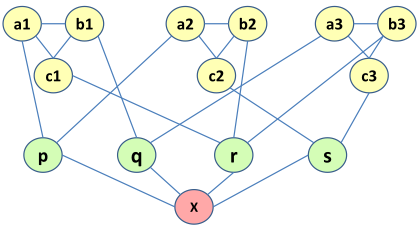
Proof Sketch. As pointed out earlier, this problem is in NP. We show that it is NP-hard by first reducing 2ROBUST 3HYPERGRAPH 2-COLORABILITY to this problem in logarithmic space, and then using Theorem 3.1. Consider a 3hypergraph H whose edges are C1, . . . , Cr. We transform H into a graph G = (V, E) as follows: The graph G contains a node p for each node p of H. Moreover, G contains a special node X that is connected to each such node p. Finally, for each 3-hyperedge Ci of H, the graph G contains a triangle Ti with fresh nodes ai, bi, ci, such that each node of Ci is connected to exactly one node of this triangle. This completes the construction of G. This is illustrated in Figure 1 for a hypergraph H having hyperedges {p, q, r}, {p, r, s}, and {q, r, s}.
Claim: H is a "yes"-instance of 2ROBUST 3-HYPERGRAPH 2-COLORABILITY if and only if G is a "yes"-instance of ROBUST GRAPH 3-COLORABILITY.
To prove the "if-direction" of the claim, assume G is a "yes"-instance of ROBUST GRAPH 3-COLORABILITY. Let p, q be two vertices of H, for which we fix a coloring f, that is, f(p) and f(q) are some given fixed colors from {0, 1}. Because of the well-known symmetry of 3-HYPERGRAPH 2COLORABILITY with respect to dual colorings, it is actually sufficient to specify whether f(p) = f(q) or f(p) ̸= f(q). We need to show that f can be extended to a correct 2-coloring f ∗ to all vertices of H. Given that G is a "yes"-instance of ROBUST GRAPH 3-COLORABILITY, there must be a 3coloring g : V (G) -→ {0, 1, 2} of G that is consistent with f , i.e., that assigns the same colors to any nodes p and q if and only if f(p) = f(q). Thus, assume g is such a 3coloring. Observe that, because of node X, all vertices of G that are also vertices of H must be colored by two colors only, say, w.l.o.g., colors from {0, 1}. Let f ∗ be the corresponding 2-coloring of the vertices of H. Obviously, f ∗ is consistent with f. It remains to show that f ∗ is effectively a correct hypergraph 2-coloring for H. Assume this is not the case. Then, for some set Ci with vertices p, q, r, f(p) = f(q) = f(r). For the corresponding nodes p, q, r, we then have g(p) = g(q) = g(r), and therefore the triangle 〈ai, bi, ci〉 would need to be colored with two colors only, which is impossible. Therefore, f ∗ is a correct 2-coloring of H that, moreover, is consistent with f , and thus H is a "yes"- instance of 2ROBUST 3-HYPERGRAPH 2-COLORABILITY. This proves the "if-direction" of the claim.
The "only-if-direction" of the claim is shown in a similar spirit, but requires a rather involved case-analysis. Due to space considerations, we have to defer it to the full paper.
Theorem 3.4 ROBUST 3SAT is NP-complete.
Proof Sketch. As pointed out earlier, this problem is in NP. We show that it is NP-hard by first reducing 3ROBUST 12SAT to this problem in logarithmic space, and then using Theorem 3.2. Let ϕ be a 12CNF formula C1 ∧ C2 ∧ · · · ∧ Cm, where each Ci is a clause of the form ℓ1i ∨ · · · ∨ ℓ12 i and each ℓji is a literal, for 1 ≤ i ≤ m and 1 ≤ j ≤ 12. For each clause Ci, let p2i , . . . p10 i be nine fresh propositional variables. Let ϕ∗ be the 3CNF formula obtained from ϕ by replacing each clause Ci by the following conjunction Γi of 3-clauses:
Note that this transformation is just a special instantiation of the well-known logarithmic-space reduction of SAT to 3SAT. Therefore it is easy to see that ϕ is satisfiable if and only if ϕ∗ is satisfiable. Here, however, we need to show that the following holds:
Claim: ϕ is a "yes" instance of 3ROBUST 12SAT if and only if ϕ∗ is a "yes" instance of ROBUST 3SAT.
The easier part is the "if-direction". Assume ϕ∗ is a "yes" instance of ROBUST 3SAT. To show that ϕ is then a "yes" instance of 3ROBUST 12SAT, take any partial truth value assignment (tva) f to three variables of ϕ. This can be extended to a total satisfying tva f + to ϕ∗ . The restriction of f to the ℓ-variables is also a satisfying tva to ϕ. This is easy to check. The "only-if-direction" of the claim, proven in detail in the full paper, is rather non-trivial. Here, we only provide a rough intuition about the technique. Assume that ϕ is a "yes" instance of 3ROBUST 12SAT. We must show that ϕ∗ is a "yes" instance of ROBUST 3SAT. The key idea is that, given a partial tva t∗ on three variables of ϕ∗ , one can transform t∗ to a carefully chosen partial tva t on three variables of ϕ, and then use the 3-robustness of ϕ to extend t to a satisfying assignment of ϕ, which, in turn, can be used to extend t∗ to a satisfying assignment of ϕ∗ .
To obtain t from t∗ , we carefully replace each truth value assignment of t∗ to a to p-variable (i.e., a propositional variable of ϕ∗ that does not occur in ϕ) by an appropriate tva to an ℓ-variable (i.e., a to variable that occur in both ϕ and ϕ∗ ). For convenience, rather than dealing with tva's to propositional variables, we consider tvas to literals. For example, rather than saying pi is assigned true, we say that literal ¬pi is assigned false (which is obviously equivalent). We obtain t from t∗ by replacing each assignment of t∗ that assigns false to a p-literal λ by an assignment that assigns true to an ℓliteral λ′ = proxy(λ), the so called the proxy of λ. Intuitively, setting proxy(λ) to true will ensure that the clause in which λ occurs is satisfied by some literal different from λ; therefore, λ can be safely set to false without endangering the overall satisfiability of φ∗ . In the simplest case, proxy(λ) is just the unique ℓ-literal in the same clause as λ. If this ℓliteral were forced to be true, then t would make the clause true, even if we assigned false to λ. But choosing this simple proxy for λ is not always possible, because this ℓ-literal itself may be required to be false by t∗ . However, we are able to show that it is actually always possible to find an appropriate proxy for each ℓ-literal λ. To this aim, we define three functions π1, π2, and π3 from the p-literals of each conjunction Γi to the ℓ-literals of the same Γi, and we prove that one of π1(λ), π2(λ), π3(λ) can always be used as proxy for λ. The functions π1, π2, and π3 are illustrated in Figure 2.
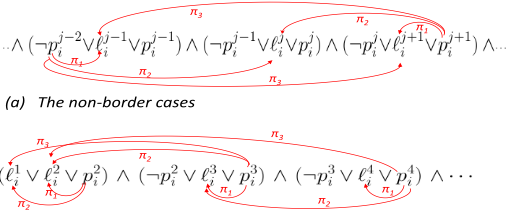
Figure 2: Candidate proxies π1, π2, and π3.
By replacing the (at most three) tvas to p-variables of the partial tva t∗ by their respective proxy-assignments, we obtain a (partial) tva t to ϕ. Since ϕ is a "yes"-instance of 3ROBUST 12SAT, we have that t can be extended to a full satisfying tva t+ of ϕ. We then prove that this assignment t+ can, in turn, be extended to a full satisfying tva t‡ of ϕ∗ that is consistent with t. This shows that ϕ∗ is a "yes"-instance of ROBUST 3SAT, which settles the "only-if-direction".
4 QuantumMechanics and Hidden Variables
Background onLocal HiddenVariables Consider the following scenario. There is some system on which measurements of various quantities can be performed. Two experimenters, Alice and Bob, can each select one of several different measurements to perform, and observe one of several different outcomes. We assume that Alice and Bob are spatially separated, and there is no communication with each other while the measurements are being performed. When measurements are selected by Alice and Bob, some corresponding outcomes will be observed. These individual occurrences or "runs" of the system are the basic events. Repeated runs allow relative frequencies to be tabulated, which can be summarized by a probability distribution. We can abstract from the probabilities themselves, and focus only on the support of the probability distributions - distinguishing those events which are possible (have non-zero probability) from those which can never happen.
Here is an example of such a support table:
| (0, 0) | (1, 0) | (0, 1) | (1, 1) | |
|---|---|---|---|---|
| (a, b) | 1 | 1 | 1 | 1 |
| (a′ , b) | 0 | 1 | 1 | 1 |
| (a, b′ ) | 0 | 1 | 1 | 1 |
| (a′ , b′ ) | 1 | 1 | 1 | 0 |
| Table 1 | ||||
In this example, Alice can select measurement settings a or a′ , and Bob can select b or b′ . Each measurement can result in an outcome of 0 or 1. We consider the joint outcomes when Alice and Bob both select measurements, and tabulate which are possible. For example, if Alice chooses measurement setting a and Bob chooses b′ , then according to the above table, the joint outcome (1, 0), i.e., outcome 1 for a and 0 for b′ , is possible, while (0, 0) is not possible.
How can such correlated outcomes be explained, given our assumption about Alice and Bob? One mechanism is to assume that there are preset values for each of the measurements which Alice and Bob can make, independently of the measurement made by the other. Such preset values are specified by functions h : {a, a′ , b, b′} → {0, 1}. We allow for the fact that there may be several possible such preset values, which are determined by circumstances beyond our control, by saying that the behaviour of the system is "covered" by a set of such functions {h1, . . . , hp}. Such a set generates a support table by the rule that an entry for measurements (x, y) and outcomes (u, v) is set to 1 if and only if for some i, hi(x) = u and hi(y) = v.
We can now ask the question: can the above support table be realized by a set of functions in such a fashion? The answer is that it cannot. This can be shown by using only the following information from the table: the joint outcome (0, 0) is possible for measurements (a, b), while the joint outcome (0, 0) is impossible for the pairs (a′ b) and (a, b′ ), and the joint outcome (1, 1) is impossible for the pair (a′ , b′ ).
What makes this fact remarkable is that the above support table can be realized physically. That is, we can generate a two-qubit quantum state, and local spin measurements for Alice and Bob corresponding to the measurements a, a′ , b, b′ , such that quantum mechanics predicts, and experiment confirms, this support table. Moreover, these predictions are verified even under conditions of spatial separation of the two subsystems corresponding to Alice and Bob. The particular construction we have described is known as Hardy's paradox [Hardy, 1993], a variant of Bell's theorem [Bell, 1964].
Thus Nature realizes non-local correlations, which do not admit any explanation in terms of values possessed by the physical quantities under consideration independently of the actual combination of measurements which are performed. Such an explanation is called a local hidden-variable model, so Hardy's paradox is showing that no such local hidden variable model exists for the empirically observed table of possible behaviours we gave above. This leads to the following natural computational problem: given a possibility table, determine whether it has a local hidden-variable model. We focus on this problem next.
Complexity of Local Hidden-Variable Models [Abramsky, 2013] introduced a relational framework for studying the notions of hidden variables and locality in quantum mechanics. Assume we have n different experimenters, for some n ≥ 1. The ith experimenter can select measurements from a set Mi of available measurements, whose possible outcomes form a set Oi, 1 ≤ i ≤ n. Let M = Πni=1Mi be the set of all combinations of available measurements, and let O = Πni=1Oi be the set of all combinations of possible outcomes. A relational model of dimension n is a relational structure of the form (M, O, e), where e ⊆ M × O.
For example, Table 1 gives rise to the relational model (M,O, e) of dimension 2, where M = M1 × M2 with M1 = {a, a′ } and M2 = {b, b′}, O = O1 × O2 with O1 = O2 = {0, 1}, and e is the relation consisting of all tuples (m1,m2, o1, o2) such that the entry in the cell determined by row (m1,m2) and column (o1, o2) is equal to 1.
In [Abramsky, 2013], the notion of a local hidden-variable model was rigorously defined and the properties of the classes HV(n) of all local hidden-variable models of dimension n were investigated. Each class HV(n) can be identified with the following decision problem, which, for simplicity, is also denoted by HV(n): Given a relational model (M,O, e) of dimension n, is it in HV(n)?
As shown in [Abramsky, 2013], for every n ≥ 1, the class HV(n) consists of all relational models (M, O, e) that satisfy the following formula Ψ(n) of second-order logic:
where the variables in x and u range over M, the variables in y range over O, and the relational symbol R is interpreted by the relation e of the model.
Going back to our example, the relational model (M, O, e) arising from Table 1 does not satisfy the formula Ψ(2). To see this and towards a contradiction, assume that it does. Since the tuple (a, b, 0, 0) belongs to e, there are functions f1 and f2 such that (i) f1(a) = 0 and f2(b) = 0; (ii) for all (m1, m2) in M, we have that (m1,m2, f1(m1), f2(m2)) belongs to e. Since (a′ , b, 0, 0) ̸∈ e, it follows that f1(a′ ) = 1. Similarly, since (a, b′ , 0, 0) ̸∈ e, it follows that f2(b′ ) = 1. Hence, (a′ , b′ , 1, 1) ∈ e, which is a contradiction, since the entry determined by row (a′ , b′ ) and column (1, 1) in Table 1 is 0.
An important consequence of the aforementioned characterization of HV (n) in terms of second-order logic is that HV(n) is in NP, for every n ≥ 1. The exact computational complexity of HV(n), however, was left as an open problem. Note that if n = 1, then HV(1) is actually first-order definable, hence it is in LOGSPACE (in fact, it is in the lower complexity class AC0). This is so because a relational model (M, O, e) of dimension 1 is in HV(1) if and only if e is total, that is, it satisfies the formula ∀x∃yR(x, y), where x ranges over M and y ranges over O.
The main result of this section is that HV(n) is NPcomplete, for every n ≥ 2. In fact, we obtain a complete picture for the complexity of the parameterized subclasses of HV(n) that also take into account the size of the domains Oi, 1 ≤ i ≤ n, of possible outcomes. More precisely, for every n ≥ 2 and every k ≥ 2, we write HV(n)/k to denote the subclass of HV(n) consisting of relational models (M, O, e) in which, for every i ≤ n, we have that |Oi| ≤ k.
Theorem 4.1 The following statements are true.
- HV(2)/2 is in NLOGSPACE.
- HV(2)/k is NP-complete, for every k ≥ 3. In particular, HV(2)/3 is NP-complete.
- HV(n)/k is NP-complete, for every n ≥ 3 and every k ≥ 2. In particular, HV(3)/2 is NP-complete.
Proof Sketch. We show that HV(2)/2 is in NLOGSPACE by using Theorem 5 in [Blass and Gurevich, 1986], which, in effect, asserts that the model-checking problem for narrow Henkin quantifiers is in NLOGSPACE. By definition, a narrow Henkin quantifier is a Henkin quantifier of the form
( ∀x1∃y1 ), where yi, for i = 1, 2, depends only on xi
and takes values from the set {0, 1}. Over relational models (M1 ×M2, O1 × O2, e) of dimension 2 in which the sets O1 and O2 of possible outcomes are of size 2, the existential second-order formula
can be expressed using narrow Henkin quantifiers, hence its model-checking problem is in NLOGSPACE. Since NLGOSPACE is closed under first-order quantification and Boolean operations, it follows that HV(2)/2 is in NLOGSPACE.
We show that HV(2)/3 is NP-complete by giving a logarithmic-space reduction of ROBUST GRAPH 3COLORABILITY to HV(2)/3, and then using Theorem 3.3. Specifically, given a graph G = (V,E), we construct in logarithmic space a relation e(G) ⊆ V × V × C × C, where C = {1, 2, 3}, consisting of the following quadruples: a quadruple (u, u, i, i), for every u ∈ V and every i ∈ C; a quadruple (u, v, i, j), for every u, v ∈ V such that (u, v) ∈ E, and for every i, j ∈ C such that i ̸= j; and a quadruple (u, v, i, j), for every u, v ∈ V such that u ̸= v, (u, v) ̸∈ E, and for every i, j ∈ C.
We now claim G is robustly 3-colorable if and only if (V × V, C × C, e(G)) is in HV(2)/3.
To prove the preceding claim, assume first that G is robustly 3-colorable; in particular, G is 3-colorable. We have to show that the relation e(G) satisfies the formula Ψ(2) that defines HV (2). First, it is obvious from the construction of e(G) that for all u and v in V , there are i and j in O such that (u, v, i, j) ∈ e(G). Next, assume that (u, v, i, j) ∈ e(G). We distinguish two cases. If u = v or if (u, v) ∈ E, then, since G is 3-colorable, there is a 3-coloring c : V ↦→ O of G such that c(u) = i and c(v) = j (to find such a 3-coloring of G, we may need to permute the colors in a given 3-coloring of G). We can then satisfy the formula Ψ(2) by putting f1 = f2 = c. If u and v are two independent nodes, then, using the robust 3-colorability of G, we can find a 3-coloring c : V ↦→ O of G such that c(u) = i and c(v) = j. As before, we can satisfy the formula Ψ(2) by putting f1 = f2 = c.
For the other direction, assume that the relation e(G) satisfies the formula Ψ(2). We have to show that the graph G = (V,E) is robustly 3-colorable. Let x and z be two independent nodes in G and let i and j be two colors in O = {1, 2, 3}. We have to show that there is a 3-coloring c of G such that c(x) = u and c(z) = j. By the construction of e(G) and since (x, z) ̸∈ E, we have that (x, z, i, j) ∈ e(G). Since e(G) satisfies Ψ(2), we have that there are functions f1 and f2 such that f1(x) = i, f2(z) = j, and, for all u, v in V , it is the case that (u, v, f1(u), f2(v)) ∈ e(G). By the construction of e(G), we have that f1(w) = f2(w), for every w ∈ V ; this is so because if the first two coordinates in a quadruple in e(G) are equal to each other, then the last two coordinates of that quadruple are equal to each other as well. Moreover, again by the construction of e(G), we have that the function f1 must be a 3-coloring of G; this is so because if the first two coordinates in a quadruple in e(G) form an edge, then the last two coordinates must be different from each other, which means that f1(u) ̸= f1(v). Using an analogous construction, we show that HV(3)/2 is NP-complete by giving a logarithmic-space reduction of ROBUST 3SAT to HV(2)/3, and then using Theorem 3.4.
The remaining cases follow easily from the preceding two NP-hardness results. Details are given in the full paper.
5 Conclusion and FutureWork
We have discovered a surprising link between constraint satisfaction and a natural problem in quantum mechanics: deciding whether a given set of measurements can be explained through local hidden variables, and may thus be explained through classical physics. We settled an open question by showing that this problem is NP-complete, and we were able to delimit the precise boundaries of NP-completeness for it. This is, to the best of our knowledge, one of the very few results that pinpoint the (classical) computational complexity of a decision problem in quantum mechanics. The only other significant result of which we are aware is due to Pitowsky [Pitowsky, 1991], and concerns a totally different problem, namely, testing a vector for membership in a correlation polytope. The connection to quantum mechanics is that certain correlation polytopes are defined by Bell inequalities [Clauser et al., 1969; Clauser and Horne, 1974].
Our results for local hidden-variable models were shown in the context of the possibilistic (non-probabilistic) relational quantum mechanical framework of [Abramsky, 2013]. It is worth commenting at this point on the significance of results that are couched in terms of the support tables of the probability distributions, rather than the probabilities themselves. As shown in [Abramsky, 2013], such results are stronger than those involving probabilities, thus no-go theorems at the possibilistic level imply those at the probabilistic level. The quantum foundations literature has many well-known examples of inequality-free or probability-free proofs of variants of Bell's theorem [Greenberger et al., 1990; Mermin, 1990; Cabello, 2001; Hardy, 1993; Zimba and Penrose, 1993], which are essentially performed at the level of the support tables. At the same time, the relational level of description brings to the fore striking and surprising connections between ideas in quantum foundations, and a number of notions which have been well-studied in Computer Science; see e.g. [Abramsky, 2012].
As a main and novel tool in obtaining our results, we used the new general concept of robust CSP, and we studied two particular robust CSPs, namely ROBUST GRAPH 3COLORABILITY and ROBUST 3SAT, that are directly relevant to the HV(n) problem of hidden-variable detection. We believe, however, that the concept of robust CSP is of interest in its own right; actually, we believe that by having studied two very specific robust CSPs here, we have only scratched the tip of an iceberg. In the near future, we plan to embark on a systematic study of robust CSPs aiming to identify general principles that govern robustness and its complexity.
Acknowledgments Samson Abramsky and Phokion Kolaitis wish to acknowledge the hospitality of the Isaac Newton Institute for Mathematical Sciences, where they had the opportunity to visit and interact during the programme Semantics and Syntax: A Legacy of Alan Turing in Arpil 2012. Samson Abramsky's work was supported by the EPSRC Senior Research Fellowship EP/E052819/1, Foundational Structures and Methods for Quantum Informatics, and by the Templeton Foundation grant, Categorical Unification. Georg Gottlob's work was supported by the EPSRC grant EP/G055114/1 Constraint Satisfaction for Configuration: Logical Fundamentals, Algorithms, and Complexity. Phokion Kolaitis' work was supported by NSF Grant IIS-1217869.
@inproceedings{ijcai2013p73,
  title     = {Robust Constraint Satisfaction and Local Hidden Variables in Quantum Mechanics},
  author    = {Abramsky, Samson and Gottlob, Georg and Kolaitis, Phokion G.},
  booktitle = {Proceedings of the Twenty-Third International Joint Conference on
               Artificial Intelligence, {IJCAI-13}},
  publisher = {AAAI Press / International Joint Conferences on Artificial Intelligence},
  editor    = {Francesca Rossi},
  pages     = {440--445},
  year      = {2013},
  month     = {8},
  url       = {https://ijcai.org/proceedings/2013/73},
}
TY - CPAPER TI - Robust Constraint Satisfaction and Local Hidden Variables in Quantum Mechanics AU - Abramsky, Samson AU - Gottlob, Georg AU - Kolaitis, Phokion G. T2 - Proceedings of the Twenty-Third International Joint Conference on Artificial Intelligence, IJCAI-13 PB - AAAI Press / International Joint Conferences on Artificial Intelligence PY - 2013 SP - 440 EP - 445 UR - https://ijcai.org/proceedings/2013/73 ER -Copied
Machine-readable versions of this paper, for tools and AI agents:





