
Socioscope: Spatio-Temporal Signal Recovery from Social Media (Extended Abstract)
Proceedings of the Twenty-Third International Joint Conference on Artificial Intelligence. Pages 3096-3099.
© 2013 International Joint Conferences on Artificial Intelligence
Abstract
Counting the number of social media posts on a target phenomenon has become a popular method to monitor a spatiotemporal signal. However, such counting is plagued by biased, missing, or scarce data. We address these issues by formulating signal recovery as a Poisson point process estimation problem. We explicitly incorporate human population bias, time delays and spatial distortions, and spatiotemporal regularization into the model to address the data quality issues. Our model produces qualitatively convincing results in a case study on wildlife roadkill monitoring.
- [Allan, 2002] James Allan. Topic Detection and Tracking: Event-Based Information Organization. Kluwer Aca- demic Publishers, Norwell, MA, 2002.
- [Becker et al., 2011] Hila Becker, Naaman Mor, and Luis Gravano. Beyond trending topics: Real-world event iden- tification on twitter. In Proceedings of the 5th Interna- tional AAAI Conference on Weblogs and Social Media, pages 438-441, Barcelona, Spain, 2011.
- [Cataldi et al., 2010] Mario Cataldi, Luigi Di Caro, and Claudio Schifanella. Emerging topic detection on twitter based on temporal and social terms evaluation. In Proceed- ings of the 10th International Workshop on Multimedia Data Mining, pages 4:1-4:10, Washington, D.C., 2010.
- [Chung, 1997] Fan RK Chung. Spectral graph theory. Regional Conference Series in Mathematics. American Mathematical Society, Providence, RI, 1997.
- [Cornec, 2010] Matthieu Cornec. Concentration inequalities of the cross-validation estimate for stable predictors. Arxiv preprint arXiv:1011.5133, 2010.
- [Donoho et al., 1996] David L Donoho, Iain M Johnstone, Gérard Kerkyacharian, and Dominique Picard. Density es- timation by wavelet thresholding. The Annals of Statistics, 24:508-539, 1996.
- [Eisenstein et al., 2010] Jacob Eisenstein, Brendan O'Connor, Noah A. Smith, and Eric P. Xing. A la- tent variable model for geographic lexical variation. In Proceedings of the 2010 Conference on Empirical Meth- ods in Natural Language Processing, pages 1277-1287, Cambridge, MA, 2010.
- [Gupte et al., 2011] Mangesh Gupte, Pravin Shankar, Jing Li, S. Muthukrishnan, and Liviu Iftode. Finding hierarchy in directed online social networks. In Proceedings of the 20th International Conference on World Wide Web, pages 557-566, Hyderabad, India, 2011.
- [Lazer et al., 2009] David Lazer, Alex (Sandy) Pentland, Lada Adamic, Sinan Aral, Albert Laszlo Barabasi, De- von Brewer, Nicholas Christakis, Noshir Contractor, James Fowler, Myron Gutmann, Tony Jebara, Gary King, Michael Macy, Deb Roy, and Marshall Van Alstyne. Life in the network: the coming age of computational social science. Science, 323(5915):721-723, 2009.
- [Mei et al., 2006] Qiaozhu Mei, Chao Liu, Hang Su, and ChengXiang Zhai. A probabilistic approach to spatiotem- poral theme pattern mining on weblogs. In Proceedings of the 15th International Conference on World Wide Web, pages 533-542, Edinburgh, UK, 2006.
- [Nocedal and Wright, 1999] Jorge Nocedal and Stephen J Wright. Numerical optimization. Springer series in op- erations research. Springer, New York, NY, 1999.
- [Patterson et al., 2007] B. D. Patterson, G. Ceballos, W. Sechrest, M. F. Tognelli, T. Brooks, L. Luna, P. Ortega, I. Salazar, and B. E. Young. Digital distribution maps of the mammals of the western hemisphere, version 3.0. Technical report, NatureServe, Arlington, VA, 2007.
- [Sakaki et al., 2010] Takeshi Sakaki, Makoto Okazaki, and Yutaka Matsuo. Earthquake shakes twitter users: real-time event detection by social sensors. In Proceedings of the 19th International Conference on World Wide Web, pages 851-860, Raleigh, NC, 2010.
- [Settles, 2011] Burr Settles. Closing the Loop: Fast, Inter- active Semi-Supervised Annotation With Queries on Fea- tures and Instances. In Proceedings of the 2011 Confer- ence on Empirical Methods in Natural Language Process- ing, pages 1467-1478, Edinburgh, UK, 2011.
- [Van Der Laan and Dudoit, 2003] Mark J Van Der Laan and Sandrine Dudoit. Unified cross-validation methodol- ogy for selection among estimators and a general cross- validated adaptive epsilon-net estimator: Finite sample or- acle inequalities and examples. U.C. Berkeley Division of Biostatistics Working Paper Series, pages 130-236, 2003.
- [Vardi et al., 1985] Y. Vardi, L. A. Shepp, and L. Kauf- man. A statistical model for positron emission tomog- raphy. Journal of the American Statistical Association, 80(389):8-37, 1985.
- [Willett and Nowak, 2007] Rebecca M Willett and Robert D Nowak. Multiscale poisson intensity and density es- timation. IEEE Transactions on Information Theory, 53(9):3171-3187, 2007.
- [Xu et al., 2012] Jun-Ming Xu, Aniruddha Bhargava, Robert Nowak, and Xiaojin Zhu. Socioscope: Spatio-temporal signal recovery from social media. In Proceedings of the 2012 European Conference on Machine Learning and Principles and Practice of Knowledge Discovery in Databases, pages 644-659, Bristol, UK, 2012.
- [Yang et al., 1998] Yiming Yang, Tom Pierce, and Jaime Carbonell. A study of retrospective and on-line event de- tection. In Proceedings of the 21st Annual International ACM SIGIR Conference on Research and Development in Information Retrieval, pages 28-36, Melbourne, Aus- tralia, 1998.
- [Yin et al., 2011] Zhijun Yin, Liangliang Cao, Jiawei Han, Chengxiang Zhai, and Thomas Huang. Geographical topic discovery and comparison. In Proceedings of the 20th In- ternational Conference on World Wide Web, pages 247- 256, Hyderabad, India, 2011.
References were extracted automatically from the PDF and may contain errors.
Full text extracted automatically from the PDF; figures, tables and equations may differ. The PDF is the version of record.
1 Introduction
Many real-world phenomena can be represented by a spatiotemporal signal: where, when, and how much. They can be characterized by a real-valued intensity function f ∈ R≥0, where the value fs,t quantifies the prevalence of the phenomenon at location s and time t. Examples include wildlife mortality, algal blooms, hail damage, and seismic intensity. Direct instrumental sensing of f is often difficult and expensive. Social media offers a unique sensing opportunity for such signals, where users act as "sensors" with posts on the target phenomenon (such as wildlife encounters). For instance, "I saw a dead crow on its back in the middle of the road."
There are at least three challenges when using social media users as sensors: (i) Social media posts are often ambiguous due to its language and brevity. This makes identifying social media posts on a target phenomenon extremely challenging. (ii) Social media users (our sensors) cannot be directed or focused or maneuvered as we wish. Their distribution depends on many factors unrelated to the sensing task at hand. (iii) Location and time stamps associated with social media posts may be erroneous or missing. Most posts do not include GPS coordinates, and self-reported locations can be inaccurate or false. Furthermore, there can be random delays between a target event and the generation of its social media post.
∗The paper on which this extended abstract is based was the recipient of the Best Paper on Knowledge Discovery Award of the 2012 European Conference on Machine Learning and Principles and Practice of Knowledge Discovery in Databases [Xu et al., 2012].
Most prior work in social media event analysis has focused on the first challenge. They were interested in identifying emerging topics, grouping posts by topics [Allan, 2002], and analyzing the spatio-temporal variation of popular topics [Mei et al., 2006; Cataldi et al., 2010; Yin et al., 2011]. Similarly, event detection aimed at identifying emerging events [Yang et al., 1998; Becker et al., 2011; Sakaki et al., 2010]. Other work used social media as a data source to answer scientific questions in linguistic, sociology and human interactions [Lazer et al., 2009; Eisenstein et al., 2010; Gupte et al., 2011].
Our work differs from past work and focuses on the latter two challenges. We are interested in a target phenomenon that is given and fixed beforehand. We further assume the availability of a (perhaps imperfect) trained text classifier to identify target posts. The main concerns of this paper are to deal with the highly non-uniform distribution of human sensors, which profoundly affects our capabilities for sensing target phenomena, and to cope with the uncertainties in the location and time stamps associated with target posts. The main contribution of the paper is a robust method for accurately estimate the spatiotemporal signal of the target phenomenon in light of these two challenges.
2 The Socioscope
Consider spatiotemporal signals of interest f defined on discrete spatiotemporal bins. For example, a bin (s, t) could be a U.S. state s on day t, or a county s at hour t. The task is to estimate fs,t from xs,t, the count of target social media posts within that bin. For simplicity, we often denote our signal by a vector f = (f1, . . . , fn)⊤ ∈ Rn≥0 , where fj is a non-negative target phenomenon intensity in source bin j = 1 . . . n. The mapping between index j and the aforementioned (s, t) is one-one and will be clear from context.
A commonly-used estimate is ̂ fs,t = xs,t, which can be justified as the maximum likelihood estimate of a Poisson model x ∼ Poisson(f). However, this estimate is unsatisfactory since the counts xs,t can be noisy: 1) there is a population bias - more target posts are generated when and where there are more social media users; 2) the location of a target post is frequently inaccurate or missing, making it difficult to assign to the correct bin; and 3) target posts can be quite sparse even though the total volume of social media is huge.
2.1 Penalized Poisson LikelihoodModel
To address these issues, we propose Socioscope, a probabilistic model that robustly recovers spatiotemporal signals from social media data.
Correcting Human Population Bias
To account for the population bias, we define an "active social media user population intensity" (loosely called "human population" below) g = (g1, . . . , gn)⊤ ∈ Rn≥0 . Let zj be the count of all social media posts in bin j, the vast majority of which are not about the target phenomenon. We assume zj ∼ Poisson(gj). Since typically zj ≫ 0, the maximum likelihood estimate ̂ gj = zj is reasonable.
Importantly, we then define the target posts intensity in j-th source bin with a link function η(fj , gj)
In this paper, we simply define η(fj, gj) = fj · gj, but other more sophisticated link functions can be used, too.
Handling Noisy and Incomplete Data
In recent data we collected from Twitter, only about 3% of tweets contain the latitude and longitude at which they were created. Another 47% contain a well-formed user selfdeclared location in his or her profile (e.g., "New York, NY"). However, such location does not automatically change while the user travels and thus may not be the true location at which a tweet is posted. The remaining 50% do not contain any location meta data. Clearly, we cannot reliably assign the latter two kinds of tweets to a spatiotemporal source bin. 1
To address this issue, we borrow an idea from Positron Emission Tomography [Vardi et al., 1985]. In particular, we define m detector bins which are conceptually distinct from the n source bins. The idea is that an event originating in some source bin goes through a transition process and ends up in one of the detector bins, where it is detected. This transition is modeled by an m × n matrix P = {Pij } where
P is column stochastic: ∑mi=1 Pij = 1, ∀j. We defer the discussion of our specific P to a case study, but we mention that it is possible to reliably estimate P directly from social media data (more on this later). Recall that the target post intensity at source bin j is η(fj, gj). We use the transition matrix to define the target post intensity hi (note that hi can itself be viewed as a link function ˜ η(f , g)) at detector bin i:
For the spatial uncertainty that we consider, we create three detector bins for each source bin. For a source bin (s, t), the first detector bin collects target posts at time t whose latitude and longitude meta data is available and in s. The second detector bin collects target posts at time t without latitude and longitude meta data, but whose user self-declared profile location is in s. The third detector bin collects target posts at time t without any location information. Note this detector bin is shared by all source bins (∗, t). For example, if we had n = 50T source bins corresponding to the 50 US states over T days, there would be m = (2 × 50 + 1)T detector bins.
1 It may be possible to recover location information from the text for some tweets, but the overall problem still exists.
Critically, our observed target counts x are now with respect to the m detector bins instead of the n source bins: x = (x1, . . . , xm)⊤. We also denote the count sub-vector for the first kind of detector bins by x(1) , the second kind x(2) , and the third kind x(3) . The same is true for the population counts z. The target counts x are modeled as independently Poisson distributed random variables:
The log likelihood factors as
where c is a constant. In (5) we treat g as given.
Poisson intensity f is non-negative, necessitating a constrained optimization problem in a maximizing likelihood procedure. It is more convenient to work with an unconstrained problem. To this end, we work with the exponential family natural parameters of Poisson. Specifically, let
Our specific link function becomes η(θj, ψj) = eθj+ψj . The detector bin intensities become hi = ∑nj=1 Pijη(θj , ψj ).
Addressing Data Scarcity
Target posts may be scarce in some detector bins. This problem can be mitigated by the fact that many real-world phenomena are spatiotemporally smooth, i.e., "neighboring" source bins in space or time tend to have similar intensities. We therefore adopt a penalized likelihood approach by constructing a graph-based regularizer. The undirected graph is constructed so that the nodes are the source bins. Let W be the n × n symmetric non-negative weight matrix. The edge weights are such that Wjk is large if j and k tend to have similar intensities. Since W is domain specific, we defer its construction to the case study.
Our graph-based regularizer applies to θ directly:
where L is the combinatorial graph Laplacian [Chung, 1997]: L = D-W, and D is the diagonal degree matrix with Djj = ∑nk=1 Wjk .
Finally, Socioscope solves the following penalized likelihood optimization problem:
where λ is a positive regularization weight.
2.2 Optimization and Parameter Tuning
We solve the Socioscope optimization problem (8) with BFGS, a quasi-Newton method [Nocedal and Wright, 1999]. We initialize θ with the following heuristic. Given counts x and the transition matrix P, we compute the least-squared projection η0 to ‖x -Pη0‖2, and force positivity by setting η0 ← max(10-4 , η0) element-wise, where the floor 10-4 ensures that log η0 > -∞. From the definition η(θ, ψ) = exp(θ + ψ), we then obtain the initial parameter
The choice of the regularization parameter λ has a profound effect on the smoothness of the estimates. Selecting these parameters using a cross-validation (CV) procedure gives us a data-driven approach to regularization. For theoretical reasons beyond the scope of this paper, we do not recommend leave-one-out CV [Van Der Laan and Dudoit, 2003; Cornec, 2010]. We construct the hold-out set by simply subsampling events from the total observation uniformly at random. This produces a partial data set of a subset of the counts that follows precisely the same distribution as the whole set, modulo a decrease in the total intensity per the level of subsampling. The complement of the hold-out set is what remains of the full dataset, and we use it as the training set. We select the λ that maximizes the (unregularized) log-likelihood on the hold-out set.
2.3 Theoretical Considerations
The natural measure of signal-to-noise in this problem is the number of counts in each bin. If we directly observe xi ∼ Poisson(hi), then the normalized error E[( xi-hi hi )2 ] = h-1 i ≈ x-1 i . So larger counts, due to larger underlying intensities, lead to small errors on a relative scale.
We recall the following minimax lower bound, which follows from the results in [Donoho et al., 1996; Willett and Nowak, 2007].
Theorem 1 Let f be a H¨older α-smooth d-dimensional intensity function and suppose we observe N events from the distribution Poisson(f). Then there exists a constant Cα > 0 such that
where the infimum is over all possible estimators. It is possible to show that our regularized estimators, with adaptively chosen bin sizes and appropriate regularization parameter settings, could nearly achieve this bound. This gives useful insight into the minimal data requirements of our methods. For example, consider just two spatial dimensions (d = 2) and α = 1 which corresponds to Lipschitz smooth functions. Then the error is proportional to N -1/2 . Note that the bound depends on the regularity of the underlying function f. As f becomes increasingly smooth (as α gets larger), we need fewer counts for the same level of error.
| (i) scaled x(1) | 14.11 |
| (ii) scaled x(1)/z(1) | 46.73 |
| (iii) Socioscope with x(1) | 0.17 |
| (iv) Socioscope with x(1) + x(2) | 1.83 |
| (v) Socioscope with x(1) , x(2) | 0.16 |
| (vi) Socioscope with x(1) , x(2) , x(3) | 0.12 |
3 A Synthetic Experiment
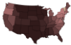
We conduct a synthetic experiment whose known groundtruth intensity f allows us to quantitatively evaluate Socioscope. With the exception of f , all settings match our case study in the next section. We design the ground-truth target signal f to be temporally constant but spatially varying. Figure 1(a) shows the ground-truth f spatially where lighter color means higher intensity. It is a mixture of two Gaussian distributions discretized at the state level. With P, g from our case study and this f , we generate the observed target post counts for each detector bin by a Poisson random number generator: xi ∼ Poisson(∑nj=1 Pi,jfjgj), i = 1 . . .m. The sum of counts in x(1) is 56, in x(2) 1106, and in x(3) 1030. Since we have 2376 detector bins, the counts are very sparse.
We compare the relative error ‖f -ˆf‖2 /‖f‖2 of several estimators in Table 1: (i) ˆf = x(1)/(ϵ1 ∑ z(1) ), where ϵ1 is the fraction of tweets with precise location stamp (discussed later in case study). Scaling matches it to the other estimators. Figure 1(b) shows this simple estimator, aggregated spatially. It is a poor estimator: besides being non-smooth, it contains 32 "holes" (states with zero intensity, colored in blue) due to data scarcity. (ii) Naively correcting the population bias by ˆf = x(1) j /(ϵ1z(1) j ) is even worse, because naive bin-wise correction magnifies the variance due to the sparsity of x(1) . (iii) Socioscope-with-x(1) -only simulates the practice of discarding noisy or incomplete data, but regularizing for smoothness. The relative error was reduced dramatically. (iv) Same as (iii) but replace the values of x(1) with x(1) + x(2) . This simulates the practice of ignoring the noise in x(2) and pretending it is precise. The result is worse than (iii), indicating that simply including noisy data may hurt the estimation. (v) Socioscope with x(1) and x(2) separately, where x(2) is treated as noisy by P. It reduces the relative error further, and demonstrates the benefits of treating noisy data specially. (vi) Socioscope with the full x. It achieves the lowest relative error among all methods, and is the closest to the ground truth (Figure 1(c)). Compared to (v), this demonstrates that even counts x(3) without location can also help us to recover f better.
4 Case Study: Roadkill
We report a case study on the spatiotemporal intensity of roadkill for several wildlife species within the continental U.S. We collected data from Twitter during September 22November 30, 2011 and aggregated them into 24 hour-of-day. Our source bins are state×hour-of-day. Let s index the 48 continental US states plus District of Columbia. Let t index
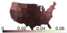

- (a) ground-truth f
- (b) scaled x(1)
- (c) Socioscope
(a) ̂g
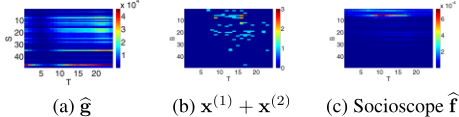
Figure 2: Raw counts and Socioscope results for chipmunks. The x-axis is hour of day and y-axis is the states, ordered by longitude from east (top) to west (bottom).
the hours from 1 to 24. This results in |s| = 49, |t| = 24, n = |s||t| = 1176, m = (2|s| + 1)|t| = 2376.
4.1 Data Preparation
Given a target post classifier and a geocoding database, it is straightforward to generate the counts x and z. As it is not the focus of this paper we omit the details here, but refer the reader to [Xu et al., 2012; Settles, 2011].
In this study, P characterizes the fraction of tweets which were actually generated in source bin (s, t) that end up in the three detector bins: precise location st(1) , potentially noisy location st(2) , and missing location t(3) . We define P as follows: P(s,t)(1) ,(s,t) = 0.03, and P(r,t)(1) ,(s,t) = 0 for ∀r ̸= s to reflect the fact that we know precisely 3% of the target posts' location. P(r,t)(2) ,(s,t) = 0.47Mr,s for all r, s. M is a 49 × 49 user declaration matrix. Mr,s is the probability that a user self-declares in her profile that she is in state r, but her post is in fact generated in state s. We estimated M from a separate large set of tweets with both coordinates and self-declared profile locations. Pt(3) ,(s,t) = 0.50. This aggregates tweets with missing information into the third kind of detector bins.
Our regularization graph has two kinds of edges. Temporal edges connect source bins with the same state and adjacent hours by weight wt, and spatial edges connect source bins with the same hour and adjacent states by weight ws. The regularization weight λ was absorbed into wt and ws. We tuned the weights wt and ws with CV on the 2D grid {10-3 , 10-2.5 , . . . , 103}2 .
4.2 Results
We present results on armadillo and chipmunk. Perhaps surprisingly, precise roadkill intensities for these animals are apparently unknown to science (this serves as a good example of the value Socioscope may provide to wildlife scientists). Instead, domain experts were only able to provide a range map of each animal, see the left column in Figure 3. These maps indicate presence/absence only, and were extracted from NatureServe [Patterson et al., 2007]. In addition, the experts defined armadillo as nocturnal and chipmunk as diurnal. Due to the lack of quantitative ground-truth, our comparison will necessarily be qualitative in nature.
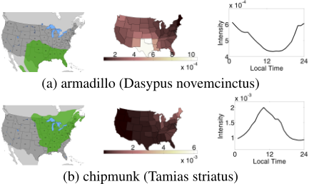
Socioscope provides sensible estimates on these animals. Figure 2(a) shows the estimated ̂g. We clearly see that human population intensity varies greatly both spatially and temporally. Figure 2(b) shows counts x(1) + x(2) for chipmunks which is very sparse (the largest count in any bin is 3), and Figure 2(c) the Socioscope estimate ̂f . In addition, we present the state-by-state intensity maps in the middle column of Figure 3 by aggregating ̂f spatially. The Socioscope results match the range maps well for these animals. The right column in Figure 3 shows the daily animal activities by aggregating ̂f temporally. These curves match the animals' diurnal patterns well, too. The Socioscope estimates are superior to the baseline methods in Table 1. The spatial and temporal patterns recovered by the baseline methods tend to have spurious peaks due to the population bias. In addition, as shown in Figure 1, they also produce many states with zero intensity due to data scarcity.
5 FutureWork
Using social media as a data source for spatiotemporal signal recovery is an emerging area. Socioscope represents a first step toward this goal. There are many open questions. For example, users may not post a squirrel encounter on the road until she arrives at home later; the local and time meta data of posts only reflect tweet-generation at home. There usually is an unknown time delay and spatial shift between the phenomenon and the post generation. Estimating an appropriate transition matrix P from social media data so that Socioscope can handle such "point spread functions" remains future work.
Acknowledgments
We thank Megan K. Hines from Wildlife Data Integration Network for providing guidance on wildlife. This work is supported in part by NSF IIS-1216758, IIS-1148012, and the Global Health Institute at the University of WisconsinMadison.
@inproceedings{ijcai2013p464,
  title     = {Socioscope: Spatio-Temporal Signal Recovery from Social Media (Extended Abstract)},
  author    = {Xu, Jun-Ming and Bhargava, Aniruddha and Nowak, Robert D. and Zhu, Xiaojin},
  booktitle = {Proceedings of the Twenty-Third International Joint Conference on
               Artificial Intelligence, {IJCAI-13}},
  publisher = {AAAI Press / International Joint Conferences on Artificial Intelligence},
  editor    = {Francesca Rossi},
  pages     = {3096--3099},
  year      = {2013},
  month     = {8},
  url       = {https://ijcai.org/proceedings/2013/464},
}
TY - CPAPER TI - Socioscope: Spatio-Temporal Signal Recovery from Social Media (Extended Abstract) AU - Xu, Jun-Ming AU - Bhargava, Aniruddha AU - Nowak, Robert D. AU - Zhu, Xiaojin T2 - Proceedings of the Twenty-Third International Joint Conference on Artificial Intelligence, IJCAI-13 PB - AAAI Press / International Joint Conferences on Artificial Intelligence PY - 2013 SP - 3096 EP - 3099 UR - https://ijcai.org/proceedings/2013/464 ER -Copied
Machine-readable versions of this paper, for tools and AI agents:





