
Short-Term Wind Power Forecasting Using Gaussian Processes
Proceedings of the Twenty-Third International Joint Conference on Artificial Intelligence. Pages 2790-2795.
© 2013 International Joint Conferences on Artificial Intelligence
Abstract
Since wind has an intrinsically complex and stochastic nature, accurate wind power forecasts are necessary for the safety and economics of wind energy utilization. In this paper, we investigate a combination of numeric and probabilistic models: one-day-ahead wind power forecasts were made with Gaussian Processes (GPs) applied to the outputs of a Numerical Weather Prediction (NWP) model. Firstly the wind speed data from NWP was corrected by a GP. Then, as there is always a defined limit on power generated in a wind turbine due the turbine controlling strategy, a Censored GP was used to model the relationship between the corrected wind speed and power output. To validate the proposed approach, two real world datasets were used for model construction and testing. The simulation results were compared with the persistence method and Artificial Neural Networks (ANNs); the proposed model achieves about 11% improvement in forecasting accuracy (Mean Absolute Error) compared to the ANN model on one dataset, and nearly 5% improvement on another.
- [Al-Yahyai et al., 2010] Sultan Al-Yahyai, Yassine Charabi, and Adel Gastli. Review of the use of numerical weather prediction (nwp) models for wind energy assessment. Re- newable and Sustainable Energy Reviews, 14(9):3192 - 3198, 2010.
- [Amjady et al., 2011] Nima Amjady, Farshid Keynia, and Hamidreza Zareipour. Short-term wind power forecast- ing using ridgelet neural network. Electric Power Systems Research, 81(12):2099 -2107, 2011.
- [C. Rasmussen, 2006] C. Williams C. Rasmussen. Gaussian Processes for Machine Learning. MIT Press, 2006.
- [Costa et al., 2008] Alexandre Costa, Antonio Crespo, Jorge Navarro, Gil Lizcano, Henrik Madsen, and Everaldo Feitosa. A review on the young history of the wind power short-term prediction. Renewable and Sustainable Energy Reviews, 12(6):1725 -1744, 2008.
- [Giorgi et al., 2011] Maria Grazia De Giorgi, Antonio Fi- carella, and Marco Tarantino. Assessment of the benefits of numerical weather predictions in wind power forecast- ing based on statistical methods. Energy, 36(7):3968 - 3978, 2011.
- [Groot, 2012] Peter Lucas Groot. Gaussian process regres- sion with censored data using expectation propagation. In Sixth European Workshop on Probabilistic Graphical Models, 2012.
- [GWEC, 2012] Global Wind Energy Council GWEC. 2012 half year report. Global Wind Report, pages 1 -8, 2012.
- [Hocaoglu et al., 2009] Fatih O. Hocaoglu, Mehmet Fidan, and Omer N. Gerek. Mycielski approach for wind speed prediction. Energy Conversion and Management, 50(6):1436 -1443, 2009.
- [Hong et al., 2010] Ying-Yi Hong, Huei-Lin Chang, and Ching-Sheng Chiu. Hour-ahead wind power and speed forecasting using simultaneous perturbation stochastic ap- proximation (spsa) algorithm and neural network with fuzzy inputs. Energy, 35(9):3870 -3876, 2010.
- [Hosansky, 2006] David Hosansky. Weather forecast accu- racy gets boost with new computer model, 2006.
- [Jiang et al., 2010] Xiaoqian Jiang, Bing Dong, Le Xie, and Latanya Sweeney. Adaptive gaussian process for short- term wind speed forecasting. In Helder Coelho, Rudi Studer, and Michael Wooldridge, editors, ECAI 2010 - 19th European Conference on Artificial Intelligence, Lis- bon, Portugal, August 16-20, 2010, Proceedings, volume 215 of Frontiers in Artificial Intelligence and Applications, pages 661-666. IOS Press, 2010.
- [Lei et al., 2009] Ma Lei, Luan Shiyan, Jiang Chuanwen, Liu Hongling, and Zhang Yan. A review on the forecast- ing of wind speed and generated power. Renewable and Sustainable Energy Reviews, 13(4):915 -920, 2009.
- [Li and Shi, 2010] Gong Li and Jing Shi. On comparing three artificial neural networks for wind speed forecasting. Applied Energy, 87(7):2313 -2320, 2010.
- [Liu et al., 2011] Heping Liu, Ergin Erdem, and Jing Shi. Comprehensive evaluation of arma arch(-m) approaches for modeling the mean and volatility of wind speed. Ap- plied Energy, 88(3):724 -732, 2011.
- [Louka et al., 2008] P. Louka, G. Galanis, N. Siebert, G. Kariniotakis, P. Katsafados, I. Pytharoulis, and G. Kal- los. Improvements in wind speed forecasts for wind power prediction purposes using kalman filtering. Jour- nal of Wind Engineering and Industrial Aerodynamics, 96(12):2348 -2362, 2008.
- [Nabney, 2004] Ian T. Nabney. Netlab: Algorithms for Pat- tern Recognition. Springer, 2004.
- [Salcedo-Sanz et al., 2009] Sancho Salcedo-Sanz, ngel M. Prez-Bellido, Emilio G. Ortiz-Garca, Antonio Portilla- Figueras, Luis Prieto, and Daniel Paredes. Hybridizing the fifth generation mesoscale model with artificial neural networks for short-term wind speed prediction. Renewable Energy, 34(6):1451 -1457, 2009.
- [Salcedo-Sanz et al., 2011] Sancho Salcedo-Sanz, Emilio G. Ortiz-Garca, ngel M. Prez-Bellido, Antonio Portilla- Figueras, and Luis Prieto. Short term wind speed predic- tion based on evolutionary support vector regression algo- rithms. Expert Systems with Applications, 38(4):4052 - 4057, 2011.
- [Soman et al., 2010] S. S. Soman, H. Zareipour, O. Malik, and P. Mandal. A review of wind power and wind speed forecasting methods with different time horizons. In Proc. North American Power Symp. (NAPS), pages 1-8, 2010.
- [Vaccaro et al., 2011] A. Vaccaro, P. Mercogliano, P. Schi- ano, and D. Villacci. An adaptive framework based on multi-model data fusion for one-day-ahead wind power forecasting. Electric Power Systems Research, 81(3):775 -782, 2011.
References were extracted automatically from the PDF and may contain errors.
Full text extracted automatically from the PDF; figures, tables and equations may differ. The PDF is the version of record.
1 Introduction
As wind is an effective renewable energy resource, the utilization of wind energy has been growing rapidly around the world. With approximately 68 GW capacity of wind farms, China has the largest wind energy generation in the world, and has continued with a high growth rate of 9% in the first half of 2012 [GWEC, 2012]. However, the intrinsically variable and uncontrollable characteristics of wind pose several operational challenges. Thus wind power prediction is an essential process for the maintenance of wind power units and energy reserve scheduling [Costa et al., 2008; Lei et al., 2009].
Short-term wind power forecasts with a prediction horizon from one hour to several days are critical to optimize wind farm maintenance and plan electricity reserves which impact grid reliability and market-based ancillary service costs. Broadly speaking, there are two approaches to short-term wind power forecasting: statistical models and physical models. The former uses only historical wind speed and power data to build statistical models, such as autoregressive integrated moving average (ARIMA) [Liu et al., 2011], Kalman filters [Louka et al., 2008], artificial neural networks [Li and Shi, 2010; Hong et al., 2010] and support vector machines [Salcedo-Sanz et al., 2011]. Since wind varies rapidly with time, the statistical models are effective only for very short-term forecasts (about 1-4 hours ahead). On the other hand, physical models have advantages over longer horizons (from several hours to dozens of hours), because they include (3D) spatial and temporal factors in a full fluid-dynamics model. However, this type of model has limitations, such as the limited observation set for calibration, the relatively limited spatial resolution possible over such a wide area, and the difficulty of accounting for local topography [Soman et al., 2010]. To overcome these limitations, some authors have combined statistical and physical models, by using NWP (Numerical Weather Prediction) data from a physical model as inputs to a statistical model [Salcedo-Sanz et al., 2009; Al-Yahyai et al., 2010].
A forecast model combined with NWP data was proposed by Vaccaro [Vaccaro et al., 2011], in which one-day-ahead wind power forecasting is realized based on information amalgamated from a local atmospheric model and measured data. Giorgi [Giorgi et al., 2011] developed a series of forecast systems by combining an Elman network and an MLP network, and predicted power production of a wind farm with three wind turbines at 5 time horizons: 1, 3, 6, 12 and 24 hours. The normalized absolute average error of the systems varied from 5.67% to 15.50% depending on forecast time and different combining ways of networks.
Recently, Gaussian Processes (GP) have been applied broadly in many domains, including wind energy prediction. Jiang and Dong focused on very short term (< 30min) windspeed prediction using GPs [Jiang et al., 2010]. They evaluated their model on real-world datasets, and found that the GP performs better than ARMA (a simpler variant of ARIMA) and Mycielski algorithms [Hocaoglu et al., 2009].
In this paper, wind-farm datasets including Numerical Weather Prediction (NWP) results and measured data from a SCADA (Supervisory Control And Data Acquisition) system are analyzed and used to develop wind power forecasting models over a horizon of up to one day, with a Gaussian Process (GP) method. The main innovations in this paper are listed below:
- The predicted wind speed from an NWP model is corrected using a GP. This process helps to improve performance compared with earlier methods for combining statistical and physical models.
- Automatic Relevance Determination was used for feature selection in order to improve generalization performance.
- A censored Gaussian Process (CGP) method is applied to build the relationship between corrected wind speed and wind power. The method accounts for the probabilistic character of the values that are not known precisely because of censoring.
- A subset of high-wind speed data is treated separately, because of its different characteristics based on analysis of the initial models.
- Historical wind speed data from the SCADA system is used as an additional input to the forecasting model for 1-4 hours-ahead prediction, since we have proved this to be effective in this range of time horizons.
Section 2 describes the NWP data used to provide daily forecasts of meteorological variables. Section 3 defines the standard and censored Gaussian Process and Automatic Relevance Determination (ARD) methods applied to build all the regression models. Section 4 describes the whole detailed modeling process from NWP data to forecast wind power results. Simulation results are presented and analyzed in Section 5. Finally, Section 6 includes the final conclusions.
2 NWPmodel and power forecasting
Numerical weather prediction uses hydrodynamic and thermodynamic models of the atmosphere to predict weather based on certain initial-value and boundary conditions. In our research, we use the WRF (Weather Research and Forecasting) NWP model. WRF was created through a partnership that includes NCAR (National Center for Atmospheric Research), NOAA (National Oceanic and Atmospheric Administration), and more than 150 other organizations and universities in the United States and internationally, and is released as a free model for public use [Hosansky, 2006].
In general, short-term wind power forecasting needs predictions from a NWP model with high spatial resolution. The data fromWRF isn't suitable directly for this application, and hence need to be interpolated both horizontally and vertically. The NWP data used in this paper is produced and interpolated from the location in the WRF model, in our case from 5kmresolution, to the accurate geographical point and hub height of each wind turbine. This prediction data is produced once each day, and is usually available at 00:00 GMT. The data including wind speed and direction, temperature, humidity and pressure, is provided at an interval of 10 minutes for the following 24 hours.
The Chinese government imposes a specific demand on the accuracy of wind power forecasting: the forecast error of 14 hours ahead should be less than 10% of wind turbine's installed capacity. All the forecast errors contained in this paper are calculated using hourly data. Therefore, we focus on forecasting with the horizon from 1 to 24 hours for wind power, based on hourly sampled NWP data.
3 Gaussian Process Methods
Gaussian processes have been successfully applied to many machine learning tasks. A systematic and detailed explanation of Gaussian process regression and Automatic Revelance Determination (ARD) can be found in Rasmussen's book [C. Rasmussen, 2006]. The extension to censored data was developed in [Groot, 2012]: here we will only provide a brief description.
3.1 Gaussian Processes
Consider a Gaussian process f(x) for a classic regression problem. Assuming we have a training set D of n observations, D = {(xi, yi)|i = 1, . . . , n}, where x denotes an input vector and y denotes a scalar output, the task is to build a function that satisfiesyi = f(xi) + ϵi. (1)
The additive noise ϵ is assumed to have a Gaussian distribution: ϵ ∼ N(0, σ2n ). Note that y is a linear combination of Gaussian variables and hence is itself Gaussian. Therefore, we have p(y|X, k) = N(0,K + σ2n I), where Kij = k(xi, xj), and the joint distribution for a new input x∗ can be written as
where k(X, x∗) = k(x∗, X)T = [k(x1, x∗), . . . , k(xn, x∗)], which we will write more briefly as k∗. Then according to the properties of joint Gaussian distributions, the prediction distribution of the target is given by a Gaussian distribution
As a result of the wind turbine control strategy, there is always a defined upper limit C and lower limit of 0 for the power generation of each turbine. Therefore, in statistical terminology, the true values (unrestricted power output) are 'censored' in that they are not observed but are replaced by the threshold value. Assuming that the latent values y∗ = f(x) can be realized by a Gaussian process, then to predict the actual output y, the influence of censoring should be considered inside the model. To implement this consideration, a censored GP model was developed in [Groot, 2012], in which the posterior distribution of y was formed by integrating out the censored distribution of latent variables and approximated using Expectation Propagation (EP). Exploratory analysis of the data shows that 5.4% percent is within 5% of the upper limit (and is thus in the range where the noise distribution overlaps significantly with the censored range). Thus it is important to account for this constraint in the model itself rather than simply pre-process the predictions of a 'standard' regression model by thresholding them at C.
3.2 Automatic Relevance Determination
As maximum likelihood can be used to determine the parameter values in the Gaussian process, we can extend this technique by incorporating a separate parameter for each input variable, the relative importance of different inputs can be inferred from the observed data [C. Rasmussen, 2006]. This leads to the Automatic Relevance Determination (ARD) method, which can be used to choose the inputs which have a significant influence on the outputs. As an example: assume the covariance function to be the squared exponential, and the original input vector has n dimensions
where all the hyperparameters can be contained in a vector θ = (θ0, L, σ2n )T , and L denotes the vector of all the parameters L = {l1, . . . , ln}. The hyperparameters {l1, . . . , ln} are used to implement ARD, since the value of li obviously determines how relevant the ith input is: as li becomes larger, the function becomes more sensitive to the corresponding input variable xi. Therefore, the importance of each input variable is revealed, and inputs with small value of li can be discarded. The ARD toolbox in Netlab [Nabney, 2004] was used to determine the appropriate inputs for each model mentioned in this paper.
4 Modeling Process
The forecasting framework proposed in this paper uses GP models and three additional features: 1. Automatic Relevance Determination (ARD) is used to select model inputs; 2. Predicted wind speed from the NWP model is corrected before modelling the mapping from wind speed to wind power; 3. Detailed adjustments were applied to improve forecast accuracy, such as including historical data and building a separate model for high wind speed.
The NWP data usually includes several meteorological variables: wind speed, wind direction, temperature, air pressure, and humidity. It is clear that wind power mainly depends on the actual wind speed, however, we don't know for sure if any other variable plays an important role too, so ARD was used to investigate the selection of input variables.
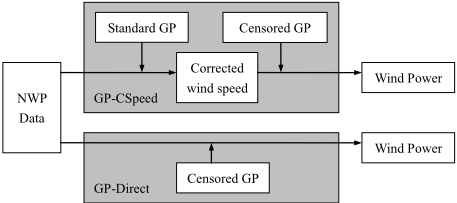
There are two ways to obtain wind power from NWP data: directly learning the model between NWP data and wind power using a censored GP; or correcting the error in NWP wind speed prediction and then building a second model for the relationship between wind speed and generated power. The second method is based on the belief, underpinned by a large body of empirical analysis, that there are some systematic and stochastic biases present in the original NWP forecasts. We denote the first way of modeling wind power as GP-direct, and the second as GP-CSpeed (meaning based on corrected speed): a simple schematic of the modeling process is shown in Figure 1.
Figure 2 shows the detailed structure of the proposed correction process. Certain constraints are used to improve the accuracy of modeling. First of all, the process provides forecasts of power from01:00GMT to 24:00GMT, from the time point of 00:00 GMT. This is because the NWP data is derived from running the model once per day (due to its computational cost). Since the character of wind changes with the diurnal cycle, the prediction error of the NWP model shows different properties depending on the forecast horizon. Therefore, we built a separate model for each one-hour forecast horizon and the training dataset is divided into 24 subsets. Secondly, as mentioned before, exploratory work showed that historical data of measured wind speed is useful for forecasting when the time horizon is less than 4 hours, and is therefore included as an input for models 1-4 (i.e. 1-4 hours forecast horizon) only. Thirdly, the prediction error of the NWP model appears to be larger and more related to humidity when the predicted wind speed is high, thus we developed independent GP models (labeled Model A1, A2 in the figure) specifically to improve the correction accuracy when the predicted wind speed is larger than H m/s, where H is dataset-dependent.
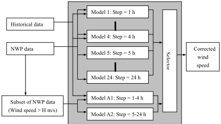
As shown in Figure 2, models 1-24 give results of correction for 1-24 hours ahead predicted wind speed, while models A1 and A2 are used to correct high NWP wind speeds. The reason for building just two models for high wind speed, is that high speed part only accounts for around 5% of the whole dataset, thus there is not enough data for training 24 high speed models separately. The 'selector' component means that when the NWP predicted wind speed is larger than H m/s, then the corresponding corrected wind speed in the result of model 1-24 is replaced by the output of model A1 or A2.
5 Experimental Validation
Two real-world datasets based on wind farms are used in this paper to evaluate our approach. The first one is from a wind farm in Gansu province (denoted as Farm-G), which is located in the windy western part of China. The other, denoted by Farm-J, is from Jiangsu province, a coastal area located in southern China. These two farms are about 2400km apart, and therefore the weather conditions are independent from each other.
| Location | Installed Capacity (kW) | Height (m) | Number |
|---|---|---|---|
| Farm-G1 | 850 | 55 | 58 |
| Farm-G2 | 1500 | 65 | 33 |
| Farm-J | 1500 | 80 | 67 |
As shown in Table 1, Farm-G is a large wind farm divided into two parts: the installed capacity of one turbine type is 850kW, and the other is 1500kW. Actually, the NWP data of Farm-G are obtained from two different models separately developed for these two groups, because of the difference in turbine height. Datasets from both farms have a time scale from April 2010 to December 2011: we have used a whole year from April 1st 2010 to April 1st 2011 as a training set, and the remainder as an independent test set.
5.1 Forecasting accuracy evaluation
Several criteria are used to evaluate the accuracy of the proposed approach. Three error measures were employed for model evaluation and model comparison: the Root Mean Square Error (RMSE), the Mean Absolute Error (MAE), and Normalized Mean Absolute Percentage Error (NMAPE). The error measures are defined as follows
where yt represents the actual observation value at time t, ˆ yt represents the forecast value for the same period, n is the number of forecasts, and the installed capacity of wind turbine is denoted by C.
We selected NMAPE as the most useful measure to interpret the quality of forecast, since this enables us to compare performance for the different type of wind turbines with variant installed capacity.
As the Government-specified accuracy requirement is NMAPE ≤ 10% for 1-4 hour-ahead forecast, we define an extra criterion to determine the performance of prediction
where m denotes the size of the corresponding test dataset.
5.2 Effectiveness of proposed model
First of all, ARD was applied to determine which NWP variables should be included as inputs to the correction model. The relevance values for measured wind speed as the target variable are shown in Table 2.
| Location | Wind- speed | Wind- direction | Temper- ature | Air pressure | Humidity |
|---|---|---|---|---|---|
| Farm-G1 | 0.2305 | 0.0000 | 0.8581 | 0.0004 | 0.0004 |
| Farm-G2 | 0.2057 | 0.0031 | 0.3142 | 0.0003 | 0.0272 |
| Farm-J | 0.0578 | 0.0001 | 0.2444 | 0.0000 | 0.0015 |
Though the specific values vary for different datasets, there is a common characteristic that the wind speed and temperature variables impact prediction accuracy the most, therefore we use these two as inputs in the GP correction process. In order to illustrate the effectiveness of the whole modeling process, we show the results for a single wind turbine from Farm-G2 as an example in Figure 3.
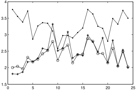
It can be clearly observed that for the short-horizon forecasts, the addition of historical data successfully reduced prediction error, but introduced additional error (probably due to overfitting) as the forecast horizon grew, especially when the forecast horizon is greater than 6. Therefore, we chose to include historical data for 1-4 hour-ahead wind speed correction only.
In order to display and analyze the performance of correction models, we first divided the dataset by NWP-predicted wind speed ˆ yt, that is Ds = {s - 1 ≤ ˆ yt < s, s = 1, 2, . . . }, then calculated the RMSE of each subset Ds, and plotted the RMSE value with s. As shown in Figure 4(a), the performance of the correction models 1-24 is good and stable when s ≤ 10, however, for higher wind speeds the corrected results become worse. On further analysis, it was noticed that humidity is more important as wind speed increases, especially for s > 13.
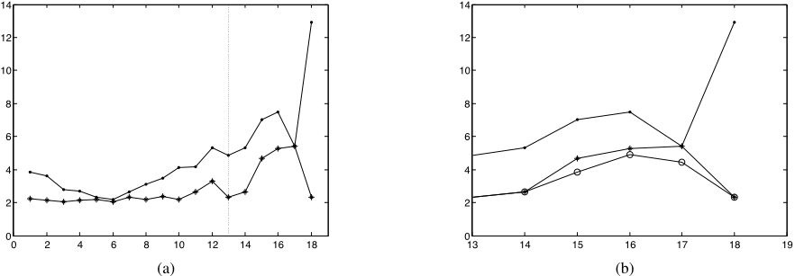
As a result, the high-speed subset is selected with a threshold H = 13 m/s for Farm-G2, and special correction models A1-2 can be built with predicted wind speed, temperature and humidity in NWP data as inputs. By the same analysis process, the threshold value is determined to be H = 12 m/s for Farm-G1, and H = 15 m/s for Farm-J. The correction results for the high-speed subset are shown in Figure 4(b), which illustrates the effectiveness of building models A1-2 for high speed data.
With the whole correction process, the corrected wind speed has a much better test-set accuracy than the original NWP wind speed predictions, as shown in Table 3.
| Data | RMSE(m/s) | MAE(m/s) | Improvement |
|---|---|---|---|
| NWP-speed | 3.3057 | 2.6303 | - |
| Corrected speed | 2.3150 | 1.8115 | 31.13% |
The improvement listed in this paper is calculated in terms of MAE, by
where Eb denotes the error of basic method used as comparison, which here is the original NWP prediction error.
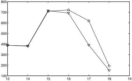
The RMSE of predicted wind power from both censored and standard GP models is calculated and the region with a high corrected wind speed s is plotted in Figure 5, because this is where the generated wind power might be censored. A standard GP can predict impossible values before being thresholded, whereas the censored GP builds the constraint into the parameter learning process. From the figure, we can clearly see that the censored and standard GPs perform equally well at medium speed, but as the wind speed grows, the difference becomes more obvious and the censored GP achieves a better performance in forecasting accuracy.
5.3 Simulation results
In this section we present the results of our power-prediction framework and some benchmarks: the persistence model and a multi-layer perceptron (MLP) neural network. The persistence method simply uses the current value as the forecast, which means that at time t, the prediction ˆ yt+1 = ˆ yt+2 = · · · ˆ yt+24 = yt. Since sometimes the wind power data may be invalid because of a turbine fault (invalid data was excluded from the dataset at the pre-processing stage), we use the current wind speed data in this model, and calculate the wind power by wind speed-power curve, which can be obtained by training historical dataset.
MLP networks have been applied to short-term wind power forecasting before, and have achieved a much better performance than the persistence method [Amjady et al., 2011], hence an MLP based model (MLP-CSpeed) which first corrects wind speed and then predicts wind power is chosen for comparison. Based on empirical results (model comparison on a validation set), the first MLP model, which corrects wind speed, used NWP wind speed, temperature and humidity as inputs, and measured wind speed as output, with a 9-neuron hidden layer. The second part of the MLP-CSpeed model used corrected wind speed as input, and has a 7-neuron hidden layer, then outputs the final prediction of wind power.
The wind turbines in Farm-G consist of two types of wind turbine, 850kW and 1500kW, and therefore we build different models for each type of turbine. Our empirical results show that one well-trained forecast model is also suitable for other turbines of the same type located at the same wind farm. The results of applying the proposed model to the test datasets are shown in Tables 4-6.
| Model | RMSE | MAE (kW) | NMAPE | Improve- P0.1 | |
|---|---|---|---|---|---|
| (kW) | ment 1 | (1-4h) | |||
| Persistence | 175.05 | 121.55 | 14.30% | - | 59.64% |
| MLP-CSpeed | 165.59 | 112.79 | 13.26% | 7.20% | 50.67% |
| GP-Direct | 173.10 | 106.49 | 12.53% | 12.40% | 66.37% |
| GP-CSpeed | 152.36 | 99.69 | 11.73% | 17.98% | 70.85% |
1. Improvement is calculated relative to the persistence method by Equation 10.
| Model | RMSE | MAE | NMAPE | Improve- P0.1 | |
| (kW) | (kW) | ment 2 | (1-4h) | ||
|---|---|---|---|---|---|
| Persistence | 356.21 | 238.27 | 15.88% | - | 60.00% |
| MLP-CSpeed | 262.75 | 188.11 | 12.54% | 21.05% | 58.14% |
| GP-Direct | 265.32 | 189.96 | 12.66% | 20.27% | 64.65% |
| GP-CSpeed | 240.69 | 166.87 | 11.02% | 30.00% | 73.02% |
2. Same as 1.
| Model | RMSE | MAE (kW) | NMAPE | Improve- P0.1 | |
|---|---|---|---|---|---|
| (kW) | ment 3 | (1-4h) | |||
| Persistence | 349.59 | 235.20 | 15.68% | - | 69.37% |
| MLP-CSpeed | 286.96 | 196.47 | 13.10% | 16.47% | 59.56% |
| GP-Direct | 288.01 | 203.12 | 13.54% | 13.64% | 59.80% |
| GP-CSpeed | 274.87 | 186.96 | 12.46% | 20.51% | 67.22% |
3. Same as 1.
As we can see from Tables 4-6, the proposed GP-CSpeed model has better performance than the other models, and especially presents a outstanding performance in 1-4 hours forecast horizon. In terms of MAE, the improvement of accuracy is 17.98%, 30.6% and 20.51% for 3 datasets. If comparing to MLP-CSpeed model, the improvement would be 11.61% for dataset of Farm-G1, 11.29% for Farm-G2, and 4.84% for Farm-J.
6 Conclusion
Short-term wind power forecasting, which strongly impacts the safety and economics of the electric grid, is an important and challenging task, considering the uncontrollable and stochastic nature of wind. In this paper, we investigated a combination of numeric and probabilistic models: a Gaussian Process (GP) combined with a Numerical Weather Prediction (NWP) model was applied to one-day-ahead wind power forecasting. Certain methods were employed to improve the forecast accuracy: predicted wind speed is firstly corrected by GP before it is used to forecast wind power; as there is a defined limit on power generation of wind turbine, a censored GP is applied to build the speed-power model; ARD is used to choose effective NWP variables as inputs to each model; for very short-term forecasts, historical data is added into modeling process; and a high wind-speed subset is treated separately by building a single forecast model.
The simulation results shows that, compared to an MLPCSpeed model, the proposed model has around 11% improvement of accuracy for the datasets of Farm-G, and 4.84% improvement for dataset of Farm-J, hence the effectiveness and performance of the GP-CSpeed model is proved.
Acknowledgments
We are thankful to the National Fund for Creative Groups of China (Grant No. 61121003), for support in the accomplishment of the present study. This work has been partially supported by the BUAA Scholarship, which funded N.C.'s visit to Aston University.
@inproceedings{ijcai2013p411,
  title     = {Short-Term Wind Power Forecasting Using Gaussian Processes},
  author    = {Chen, Niya and Qian, Zheng and Nabney, Ian T. and Meng, Xiaofeng},
  booktitle = {Proceedings of the Twenty-Third International Joint Conference on
               Artificial Intelligence, {IJCAI-13}},
  publisher = {AAAI Press / International Joint Conferences on Artificial Intelligence},
  editor    = {Francesca Rossi},
  pages     = {2790--2795},
  year      = {2013},
  month     = {8},
  url       = {https://ijcai.org/proceedings/2013/411},
}
TY - CPAPER TI - Short-Term Wind Power Forecasting Using Gaussian Processes AU - Chen, Niya AU - Qian, Zheng AU - Nabney, Ian T. AU - Meng, Xiaofeng T2 - Proceedings of the Twenty-Third International Joint Conference on Artificial Intelligence, IJCAI-13 PB - AAAI Press / International Joint Conferences on Artificial Intelligence PY - 2013 SP - 2790 EP - 2795 UR - https://ijcai.org/proceedings/2013/411 ER -Copied
Machine-readable versions of this paper, for tools and AI agents:





