
An Admissible Heuristic for SAS+ Planning Obtained from the State Equation
Proceedings of the Twenty-Third International Joint Conference on Artificial Intelligence. Pages 2268-2273.
© 2013 International Joint Conferences on Artificial Intelligence
Abstract
Domain-independent optimal planning has seen important breakthroughs in recent years with the development of tractable and informative admissible heuristics, suitable for planners based on forward state-space search. These heuristics allow planners to optimally solve an important number of benchmark problems, including problems that are quite involved and difficult for the layman. In this paper we present a new admissible heuristic that is obtained from the state equation associated to the Petri-net representation of the planning problem. The new heuristic, that does not fall into one of the four standard classes, can be computed in polynomial time and is competitive with the current state of the art for optimal planning, as empirically demonstrated over a large number of problems, mainly because it often shows an improved quality-to-cost ratio. The new heuristic applies to SAS+ planning tasks with arbitrary non-negative action costs.
- [Bonet and Geffner, 2001] B. Bonet and H. Geffner. Plan- ning as heuristic search. AIJ, 129(1-2):5-33, 2001.
- [Bonet and Helmert, 2010] B. Bonet and M. Helmert. Strengthening landmark heuristics via hitting sets. In Proc. ECAI, pages 329-334, 2010.
- [Coles et al., 2008] A. Coles, M. Fox, D. Long, and A. Smith. Additive-disjunctive heuristics for optimal plan- ning. In Proc. ICAPS, pages 44-51, 2008.
- [Domshlak et al., 2012a] C. Domshlak, E. Karpas, and S. Markovitch. Online speedup learning for optimal plan- ning. JAIR, 44:709-755, 2012.
- [Domshlak et al., 2012b] C. Domshlak, M. Katz, and S. Lefler. Landmark-enhanced abstration heuristics. AIJ, 189:48-68, 2012.
- [Edelkamp, 2001] S. Edelkamp. Planning with pattern databases. In Proc. ECP, pages 13-24, 2001.
- [Haslum and Geffner, 2000] P. Haslum and H. Geffner. Ad- missible heuristic for optimal planning. In Proc. AIPS, pages 140-149, 2000.
- [Haslum et al., 2007] P. Haslum, A. Botea, M. Helmert, B. Bonet, and S. Koenig. Domain-independent construc- tion of pattern database heuristics for cost-optimal plan- ning. In Proc. AAAI, pages 1007-1012, 2007.
- [Helmert and Domshlak, 2009] M. Helmert and C. Domsh- lak. Landmarks, critical paths and abstractions: What's the difference anyway? In Proc. ICAPS, pages 162-169, 2009.
- [Helmert et al., 2007] M. Helmert, P. Haslum, and J. Hoff- mann. Flexible abstraction heuristics for optimal sequen- tial planning. In Proc. ICAPS, pages 176-183, 2007.
- [Hickmott and Sardiña, 2009] S. L. Hickmott and S. Sardiña. Optimality properties of planning via Petri net unfolding: A formal analysis. In Proc. ICAPS, pages 170-177, 2009.
- [Hickmott et al., 2007] S. Hickmott, J. Rintanen, S. Thiébaux, and L. White. Planning via Petri net unfolding. In Proc. IJCAI, pages 1904-1911, 2007. IJCAI
- [Hoffmann and Nebel, 2001] J. Hoffmann and B. Nebel. The FF planning system: Fast plan generation through heuris- tic search. JAIR, 14:253-302, 2001.
- [Hoffmann et al., 2004] J. Hoffmann, J. Porteous, and L. Se- bastia. Ordered landmarks in planning. JAIR, 22:215-278, 2004.
- [Karpas and Domshlak, 2009] E. Karpas and C. Domshlak. Cost-optimal planning with landmarks. In Proc. IJCAI, pages 1728-1733, 2009. IJCAI
- [Katz and Domshlak, 2008] M. Katz and C. Domshlak. Structural patterns heuristics via fork decomposition. In Proc. ICAPS, pages 182-189, 2008.
- [Korte and Vygen, 2001] B. Korte and J. Vygen. Combina- torial Optimization: Theory and Algorithms (2nd Edition). Springer, Berlin, Germany, 2001.
- [Murata, 1989] T. Murata. Petri nets: Properties, analysis and applications. Proceedings of the IEEE, 77(4):541- 580, 1989.
- [Richter and Westphal, 2010] S. Richter and M. Westphal. The LAMA planner: Guiding cost-based anytime planning with landmarks. JAIR, 39(1):127-177, 2010.
- [van den Briel et al., 2007] M. van den Briel, J. Benton, S. Kambhampati, and T. Vossen. An LP-based heuristic for optimal planning. In Proc. CP, pages 651-665, 2007.
- [Zhu and Givan, 2003] L. Zhu and R. Givan. Landmark ex- traction via planning graph propagation. In ICAPS Doc- toral Consortium, pages 156-160, 2003.
References were extracted automatically from the PDF and may contain errors.
Full text extracted automatically from the PDF; figures, tables and equations may differ. The PDF is the version of record.
1 Introduction
Domain-independent planning deals with the development of planners for solving unknown input problems that are specified in a high-level description language. Domainindependent means that the planner has not other information about the problem than the one it can infer from its description. The general interest is on building "satisficing" planners whose task is to compute a valid solution, while "optimal" planners are required to output solutions of minimum cost.
Helmert and Domshlak [2009] observed that most of the well-known heuristics for optimal (and also for satisficing) planning fall in one of four categories: delete-relaxation heuristics that try to estimate the optimal cost h+ of the delete-relaxed problem [Bonet and Geffner, 2001; Hoffmann and Nebel, 2001; Coles et al., 2008], abstraction heuristics that correspond to the optimal costs of a simplified yet informative abstraction of the problem [Edelkamp, 2001; Haslum et al., 2007; Helmert et al., 2007; Katz and Domshlak, 2008], heuristics based on critical paths such as the family hm [Haslum and Geffner, 2000], and landmark heuristics that compute sets of facts or actions that every plan must achieve or execute from which the cost of an optimal plan can be estimated [Hoffmann et al., 2004; Richter and Westphal, 2010; Karpas and Domshlak, 2009; Helmert and Domshlak, 2009; Bonet and Helmert, 2010]. Currently, the most successful heuristic is the LM-cut heuristic [Helmert and Domshlak, 2009] that approximate h+ quite well on some domains, but that can also be thought as a cost-partitioning heuristic or as a landmark heuristic. LM-cut is always bounded by h+ and hence, ineffective at assessing the need to apply a fixed action multiple times for reaching the goal from a given state. On the other hand, abstraction heuristics are not delete-relaxation heuristics and have the potential to overcome this and other limitations [Helmert and Domshlak, 2009], yet to this date, the full potential of such heuristics have not been realized in a domain-independent manner and thus do not stand out as the best general heuristics.
Recent years have witnessed a remarkably progress in optimal planning in terms of the type and size of problems that can be dealt with. Current state-of-the-art optimal planners perform forward search in state space using A* with an admissible heuristic in order to meet the optimality requirement, and thus the basic difference between optimal planners is the heuristics that are used to guide the search. 1
1 More recently, best optimal planners correspond to systems that use a 'portfolio' of heuristics that are scheduled according to features of the input problem. However, a portfolio is a collection of base heuristics and hence its intrinsic limitations is a function of the heuristics in the portfolio.
In this paper we define a new heuristic for optimal planning that targets problems specified in SAS+ involving multivalued variables, arbitrary action costs, but without conditional effects. This is a class of problems that subsumes STRIPS and is as general as the classes of problems handled by other state-of-the-art heuristics. The heuristic is simple to formulate and is related to the so-called state equation for the Petri-net that is obtained from the planning problem in a standard way. For computing it, though, a small and simple linear programming problem needs to be solved. Despite the overhead involved in this computation, the new heuristic is competitive with the best current heuristics, and in some domains, it is able to solve more problems than any other heuristic. This is due to an improved quality-to-cost ratio on some domains, as observed in our experiments. We also mention how the new heuristic can be improved in three different and independent ways by either automatically reformulating the problem instance, by analyzing the resulting Petri-net of the problem, or by incorporating information from the landmarks of the problem into the linear program that defines the heuristic. The contribution of the paper thus sets a general framework for obtaining heuristics that appears to be quite promising.
The paper is organized as follows. In the next section, we present the planning framework and the concepts of Petri nets that are related to the heuristic. The new heuristic and its properties are then defined, while the experimental study and a discussion appear at the end of the paper.
2 Preliminaries
2.1 SAS+ Planning
A SAS+ problem with action costs is a tuple P = 〈V,A, sinit, sG, c〉 consisting of a set of multi-valued variables V , where each variable X ∈ V has a finite domain DX, together with a finite set A of actions, an initial state sinit, a goal description sG, and non-negative action costs c : A → N. A state in SAS+ is a V -valuation while a partial state is a partial valuations on variables; for a partial valuation ν, we use V ars(ν) to denote the set of variables that ν assigns a value, and ν|W to denote the partial valuation obtained by restricting ν to the set of variables W ∩ V ars(ν). The initial state sinit is a complete V -valuation while sG is a partial valuation that tells what are the requirements that any valid plan must achieve. Each action a ∈ A consists of a precondition and a postcondition, both corresponding to partial states and denoted by pre(a) and post(a) respectively, that specify the conditions that must hold for the action to be executable and the conditions that will hold after the execution of the action.
The state that results after applying the action a in state s is denoted by res(a, s) (always assuming that a is applicable at s), and the state that results after applying a sequence 〈a1, . . . , an〉 of actions in state s is denoted by res(〈a1, . . . , an〉, s) (always assuming that ak is applicable at res(〈a1, . . . , ak-1〉, s) for 1 ≤ k < n). We say that a partial valuation ν is reachable iff there is a sequence π = 〈a1, . . . , an〉 of actions applicable at sinit such that res(π, sinit)|V ars(ν) = ν. In particular, a state s is reachable if there is a sequence π such that res(π, sinit) = s.
A plan for problem P is a sequence π of actions that reaches sG, while its cost is the sum of the costs of the actions in π. A plan π is optimal iff it is a plan of minimum cost.
2.2 Petri Nets
A Petri net (also called place/transition or P/T net) is a type of directed graph that represents a transition system in factored form, together with an initial state called the initial marking. Petri nets had been used extensively to model and reason about concurrent and distributed systems, verification, dataflows and workflows, formal languages, etc., and more recently also automated planning [Hickmott et al., 2007; Hickmott and Sardi˜na, 2009]. Murata [1989] gives an excellent introduction to Petri nets and the most important techniques for analyzing them.
A P/T net is a directed bipartite graph between two types of nodes called places and transitions, while a marking assigns to each place a non-negative integer. If a marking assigns the integer k ≥ 0 to a place p, we say that p is marked with k tokens. Transitions represent events that map markings into markings by moving tokens from one place to another. Formally, a P/T net is a tuple PN = 〈P, T, F,W,M0〉 where P = {p1, p2, . . . , pm} and T = {t1, t2, . . . , tn} are the finite sets for places and transitions, F ⊆ (P × T) ∪ (T × P) is a set of arcs that is often called the flow relation of the net, W : F → N∗ assigns positive weights to arcs in the flow, and M0 : P → N is the initial marking of the net. The structure of the net is the tuple N = 〈P, T, F,W〉 made of the first 4 elements and represent the transition system detached of the initial marking.
The initial marking M0 of the net evolves as transitions becomes enabled and fired according to the following rules:
- Marking M enables transition t if for each arc (p, t) ∈ F, the number of tokens consumed by t from place p is at most the number of tokens assigned by M at p; i.e., W(p, t) ≤ M(p).
- Firing an enabled transition t in marking M yields a new marking M ′ that results of consuming (subtracting) W(p, t) tokens from place p, for each (p, t) ∈ F, and producing (adding) W(t, q) tokens to place q, for each (t, q) ∈ F .
If the transition t is enabled by marking M and yields markingM ′ when fired, we write M[t〉M ′ . In this case, M ′ is the marking that assigns M ′ (p) = M(p)+W(t, p)-W(p, t) tokens at place p. 2 Inductively, we writeM1[u1u2 · · · uk〉Mk+1 when transition ui is enabled by marking Mi and yields marking Mi+1 given by Mi+1(p) = Mi(p) + W(t, p) - W(p, t), for each place p ∈ P and 1 ≤ i ≤ k. An ordinary net is one in which W(·, ·) ranges over {0, 1}. Throughout the rest of the paper, we only consider ordinary nets.
If there is a sequence of transitions σ = u1 · · · uk such that M[σ〉M ′ , we say that M ′ is reachable from M through the firing sequence σ. A basic decision problem for P/T nets is to determine whether a given marking M is reachable from the initial marking M0. This is the reachability problem for P/T nets. Another related problem is the coverability problem that asks to determine whether for a given marking M, there is a marking M ′ reachable from M0 such that M(p) ≤ M ′ (p) for each place p; in the latter case, we just write M ≤ M ′ .
If every reachable marking M fromM0 (including M0 itself) assigns at most k tokens to every place, we say that the net is k-bounded. The case for k = 1 is frequent and 1bounded is commonly referred to as 1-safe or just safe.
We now present the state equation that expresses the relation between two markings M and M ′ , through a transition t when M[t〉M ′ holds, with an algebraic equation over vectors. For this, let us define the incidence matrix A = (aij) for the flow relation; it is a matrix of dimension n×m (where n and m are the number of transitions and places) given by entries
2 Strictly speaking, this is an abuse of notation as W may be undefined on some pairs, yet this is fixed by defining W(t, p) = 0 (resp. W(p, t) = 0) when (t, p) /∈ F (resp. (p, t) /∈ F).
that quantify the net change on the number of tokens at place pj caused by firing the transition ti. If we associate with transition t = ti, the control (column) vector u of dimension m × 1 given by u(j) = 1 if j = i and u(j) = 0 otherwise, then the relation M[t〉M ′ holds for two markings M and M ′ iff M(p) ≥ W(p, t) for each place p ∈ P, and M ′ = M + AT u. In particular, the latter condition is necessary for M[t〉M ′ to hold, and it can be generalized over arbitrary firing sequences σ = u1u2 · · · uk. Indeed, if we let ui to also denote the control vector of the transition that it represents, then the condition becomes M[σ〉M ′ only if
Thus, a necessary condition for M to be reachable from the initial marking M0 is that the linear system AT x = ΔM, for ΔM = M -M0, has solution x over the non-negative integers. Such a vector x is called a firing-count vector and tells how many times each transition needs to fire in order to reach M from M0. For coverability, the condition is that AT x ≥ ΔM must have solution x over the non-negative integers. Intuitively, the Equation 2 is a balance equation for flows that go through the places of the net, saying that the net change between two markings, one accessible from the other, must be an exact match of the difference between what is produced and consumed by the sequence, at each place.
2.3 Petri Nets for SAS+ Planning
A SAS+ planning problem P = 〈V, A, sinit, sG, c〉 is readily mapped into a P/T net PN = 〈P, T, F,W,M0〉 where the places are all atoms of the form 'X = x' for variable X and value x ∈ DX, and the transitions correspond to the actions a in A. The flow relation F includes the pairs (p, a) for atoms p = 'X = x' and actions a such that X ∈ V ars(pre(a)) and pre(a)[X] = x, and pairs (a, p) such that X ∈ V ars(post(a)) and post(a)[X] = x. The function W assigns unit weight to each pair in F, while M0 is the marking Msinit associated with the initial state sinit. In general, the marking Ms associated with a state s is the marking that puts one token at each place p = 'X = x' whenever s[X] = x, and puts zero tokens at the other places. The idea is to obtain a P/T net whose reachable markings M encode the reachable states s in the planning problem in such a way that M = Ms. However, this straightforward mapping does not always result in a faithful encoding of the planning problem because the resulting P/T net may not be 1-safe, meaning that a reachable marking may put 2 or more tokens at a place thus destroying the 1-1 correspondence between markings and states. In particular, there may be reachable markings M that do not stand for any reachable state either because M puts more than one token at a place, or because M puts a non-zero number of tokens at two places p = 'X = x' and q = 'X = x′ ' with x ̸= x′ . However, the following result always hold:
Theorem1. Let P = 〈V,A, sinit, sG, c〉 be a SAS+ planning problem and PN = 〈P, T, F,W,M0〉 be the P/T net associated to it. An action sequence π is applicable at the initial state sinit only if π is a firing sequence for the initial marking M0. Moreover, if π reaches the state s from sinit, then the marking M reached by π covers the marking Ms; that is, M is such that M0[π〉M and Ms ≤ M.
Proof. Both claims are proved by induction on the length π. Along the induction, one shows (simultaneously) 1) if π is applicable at sinit, π is a firing sequence for M0, and 2) if s = res(π, sinit) and M0[π〉M, then Ms ≤ M.
This theorem is important as it will allow us to prove the admissibility of the new heuristic based on the state equation.
3 The SEQHeuristic
Let π be an action sequence that achieves the state s from sinit with s satisfying the goal (i.e., s[X] = sG[X] for each variable X ∈ V ars(sG)). The firing-count vector uπ for π is the n-dimensional column vector uπ in which uπ(i) is the number of times that the i-th action in P appears in the sequence π. By the state equation and Theorem 1, π is a firing sequence for M0 and
where M is the marking generated by firing π on M0, and Ms and MsG are the markings associated with s and sG respectively. On the other hand, the cost of π can be expressed as cT uπ = ∑ni=1 c(i)uπ(i) where c is the vector of action costs such that c(i) is the cost of the i-th action.
Therefore, if x is a non-negative integer solution of the linear system AT x ≥ MsG -M0 with minimum cT x cost, then cT x ≤ cT uπ as uπ is a non-negative integer solution of the same system. On the other hand, if AT x ≥ MsG -M0 has no solution, then there is no sequence π that achieves the goal sG from the initial state sinit. These two properties are sufficient to define an admissible heuristic hiSEQ for SAS+ planning that is defined for state s as the minimum cost cT x of any non-negative integer solution x for AT x ≥ MsG - Ms. Clearly, this heuristic is not an abstraction heuristic as it is defined in terms of the whole planning problem. Also, it is not a delete-relaxation heuristic as it considers the positive and negative effects of the actions (or postconditions for actions in SAS+), and indeed, it may even infer that an action must be applied multiple times in order to reach the goal from a given state s. However, the heuristic hiSEQ is not computable in polynomial time as it involves the solution of an integer linear program. Yet, we overcome this limitation by approximating hiSEQ with the solution of the relaxed LP problem in which the integrality constraints are dropped. Hence,
Definition and Theorem 2. The hSEQ heuristic for SAS+ planning is the function that assigns the state s the value ⌈cT x∗ ⌉, where x∗ is the solution of the LP problem
if the LP has a feasible solution, and ∞ if the LP is not feasible; the case of unbounded solutions is not possible. Then, hSEQ is an admissible heuristic for SAS+ planning.
We now discuss improvements to the base hSEQ heuristic that can be implemented in a domain-independent manner.
3.1 Improvements
We report the coverage and performance for the base hSEQ heuristic in the next section. In summary, the heuristic is competitive with the best heuristics across several domains, but shows degraded performance on other domains. In this section we propose three different methods to improve the quality of the heuristic. The methods consist in either reformulating the planning problem, analyzing its safeness properties, or using the information contained in the action landmarks.
Reformulations
Problems with few goals generate goal markings MsG that have few non-zero entries. These markings result on weak constraints for the LP that yield solutions x∗ that may be ineffective to guide the search. One way to increase the value of the heuristic is to add atoms to the goal that must hold along the other conditions originally specified. For example, if the goal contains the atom X = x, which is not true initially, and every action that makes X = x true also makes Y = y true, and no other action destroys Y = y, then the planning problem can be modified without loosing any solution by extending the goal with the atom Y = y.
This idea is illustrated in the experiments where a slight change in the airport instances (done manually) increases the number of problems solved by 72.7% from 22 to 38.
Analysis of Safeness
As mentioned before, a P/T net is safe if no reachable marking assigns two or more tokens to a single place. In such a case, the reachable markings of the net are in 1-1 correspondence with the reachable states of the planning problem, and some of the inequalities in the LP problem can be tightened up to equalities. Indeed, for every place p in the P/T net for which MsG (p) = 1 (i.e. p refers to an atom of the form X = x such that sG[X] = x), we can safely enforce the constraint ATp x = MsG (p) -Ms(p) in the LP, where ATp is the row of the matrix AT for place p and s is the state on which the heuristic is being computed. The proof that this constraint can be added without loss of admissibility becomes obvious once it is observed that for safe nets, the first inequality in (3) is indeed an equality, by the correspondence between states and markings, and so for the second inequality for the coordinate referring to atom p since MsG (p) = 1 and all reachable markings are 1-bounded.
As shown by Hickmott et al. [2007], a planning problem P can be reformulated in a domain-independent manner into an equivalent problem P ′ whose P/T net is safe. This is a possible method to tighten up the LP that defines the SEQ heuristic, but the method is exponential in the maximum of |V ars(post(a)) \ V ars(pre(a))| when a ranges over all actions in the planning problem.
However, it is possible to define a restricted notion of safeness and then tighten up the inequalities using this notion. We say that a subset S of places is safe or 1-bounded for a P/T net PN if no reachable marking M puts more than one token at any place in S; i.e., M(p) ≤ 1 for each p ∈ S. By applying the above argument to the places in S, we can safely change by equalities all the inequalities for places p that are in a safe subset S and for which MsG (p) = 1. Indeed, Theorem 3. Let P and PN be a planning problem and its corresponding P/T net. Let S be a subset of places that is safe and let s be a state for the planning problem. Then, the following LP gives an admissible estimate for the state s:
where VG = V ars(sG) is the set of variables mentioned in the goal. That is, if the LP is feasible and x∗ is a solution, ⌈cT x∗ ⌉ is an admissible estimate for the cost of any plan for s; if the LP is unfeasible, there is no plan for s and the estimate ∞ is admissible; lastly, the LP cannot be unbounded.
Checking or finding safe sets S in a general P/T net is not an easy task. However, our P/T nets comes from SAS+ problems and thus it is natural to consider the set SX of places for variable X, defined by SX = {X = x : x ∈ DX}, as good candidates for safe sets. Moreover, the test to determine whether SX is safe or not is performed on the planning problem and not on the P/T net: SX is safe if every action that affects X has a precondition on X; i.e., there is no action a such that X ∈ V ars(post(a)) \ V ars(pre(a)).
Landmarks
hSEQ estimates the costs of the actions needed to cause a net change of MsG (p) -Ms(p) between the goal and the state s, for each place p. When the goal contains an atom X = x that is true at the state s, the right-hand side of the constraint for the place p = 'X = x' is zero and the constraint plays a minor role in the LP (unless the atom X = x is destroyed by another action enforced by the constraints in the LP). A similar situation appears when X = x is a prevail condition of an action a since then the transition for a consumes and produces p causing a zero net effect on it. However, if we infer that the goal X = x needs to be destroyed and re-established by any plan for state s, or that a prevail condition of such an action must be necessarily established by some other action, then we can add an additional constraint of the form
where the transitions {t1, t2, . . . , tk} correspond to all the actions that have X = x as an effect. In either case, such a set of transitions correspond to an action landmark for the planning problem. In general, an action landmark for state s is a set L of actions such that every plan for s must execute at least one action in L. Landmarks are the basis of the current state-of-the-art planners, either satisficing or optimal; they provide crucial information for the computation of heuristics and the serialization of goals and subgoals [Richter and Westphal, 2010], and there are many ways to compute them [Hoffmann et al., 2004; Zhu and Givan, 2003].
If we are given a collection of landmarks for state s, we can add one constraint for each landmark L in the collection. The resulting LP (and also ILP) is guaranteed to deliver admissible estimates for the cost of an optimal plan for s. Recently, landmarks had been used to strengthen abstraction heuristics in a similar way [Domshlak et al., 2012b]. In the experiments below, we did not test the use of landmarks to improve the heuristic.
| Domain | hLM-cut | hLM-cut ours | hLA | hM&S | HSP∗F | hSEQ | hSEQ safe |
|---|---|---|---|---|---|---|---|
| Airport (50) | 38 | 35 | 24 | 16 | 15 | 22 | 23 |
| Blocks (35) | 28 | 28 | 20 | 18 | 30 | 28 | 28 |
| Depot (22) | 7 | 7 | 7 | 7 | 4 | 6 | 6 |
| Driverlog (20) | 14 | 14 | 14 | 12 | 9 | 11 | 11 |
| Freecell (80) | 15 | 15 | 28 | 15 | 20 | 30 | 30 |
| Grid (5) | 2 | 2 | 2 | 2 | 0 | 2 | 2 |
| Gripper (20) | 6 | 6 | 6 | 7 | 6 | 7 | 7 |
| Logistics-2000 (28) | 20 | 20 | 20 | 16 | 16 | 16 | 16 |
| Logistics-1998 (35) | 6 | 6 | 5 | 4 | 3 | 3 | 3 |
| Miconic-STRIPS (150) | 140 | 140 | 140 | 54 | 45 | 50 | 50 |
| MPrime (35) | 25 | 24 | 21 | 21 | 8 | 21 | 21 |
| Mystery (19) | 17 | 17 | 15 | 14 | 9 | 15 | 15 |
| Openstacks-STRIPS (30) | 7 | 7 | 7 | 7 | 7 | 7 | 7 |
| Pathways (30) | 5 | 5 | 4 | 3 | 4 | 4 | 4 |
| Pipesworld-no-tankage (50) | 17 | 17 | 17 | 20 | 13 | 15 | 15 |
| Pipesworld-tankage (50) | 11 | 11 | 9 | 13 | 7 | 9 | 9 |
| PSR-small (50) | 49 | 49 | 48 | 50 | 50 | 50 | 50 |
| Rovers (40) | 7 | 7 | 6 | 6 | 6 | 6 | 6 |
| Satellite (36) | 8 | 9 | 7 | 6 | 5 | 6 | 6 |
| TPP (30) | 6 | 6 | 6 | 6 | 5 | 8 | 8 |
| Trucks (30) | 10 | 9 | 7 | 6 | 9 | 10 | 10 |
| Zenotravel (20) | 12 | 12 | 9 | 11 | 8 | 9 | 9 |
| Airport-modified (50) | na | 36 | na | na | na | 38 | 38 |
| Total (w/o Airport-modified) | 450 | 446 | 422 | 314 | 279 | 335 | 336 |
| Domain | hLM-cut ours | hSEQ | hSEQ safe |
|---|---|---|---|
| Elevators-08-STRIPS (30) | 19 | 9 | 9 |
| Openstacks-08-STRIPS (30) | 19 | 16 | 16 |
| Parcprinter-08-STRIPS (30) | 22 | 28 | 28 |
| Pegsol-08-STRIPS (30) | 27 | 26 | 27 |
| Scanalyzer-08-STRIPS (30) | 15 | 12 | 12 |
| Sokoban-08-STRIPS (30) | 28 | 17 | 17 |
| Transport-08-STRIPS (30) | 11 | 9 | 9 |
| Woodworking-08-STRIPS (30) | 15 | 12 | 12 |
| Total | 156 | 129 | 130 |
4 Experiments
We implemented hSEQ within the Fast Downward system, that also implements the LM-cut heuristics, and performed experiments on Xeon 5140 'Woodcrest' CPUs running at 2.33GHz and with 2GB of memory, with a cutoff time of 30 minutes. The results for other heuristics were obtained under similar circumstances and are taken from [Helmert and Domshlak, 2009]. For solving LPs, we tried three publicly available solvers: LPSOLVE, the GNU LP Kit library, and CLP. All libraries produced similar results, yet there are some discrepancies on the efficiency of the solvers, with no one dominating the others across all the problems in the benchmark. The results reported here were obtained with the CLP library.
Table 1 shows coverage results per domain for state-of-theart heuristics for optimal planning. The data for the two hSEQ columns and for the hLM-cut ours column was obtained by us. The last column refers to the heuristic hSEQ improved with the safeness information that is automatically extracted from the planning problem as described above. Table 2 shows similar coverage results for the IPC-08 domains where action costs are not uniform. The SEQ heuristic is not dominated by any other heuristic, in terms of coverage for neither set of problems, and is competitive with the best heuristics (and more, if the 150 instances of Miconic are carefully re-considered). On the other hand, hSEQ is able to solve two instances of Freecell and two of TPP that had no been reported before, and in the IPC-08 benchmarks, it performs quite well on parcprinter. The overall impact of the improvement provided by the safeness information is also shown in the tables; the difference is little because the improved LP very often provides the same estimates. To test the reformulation method for improving the heuristic, we manually changed the airport domain by simply extending the goal description with the fluent (at-segment ?a ?s) for each occurrence of the fluent (is-parked ?a ?s) in the goal, and with the fluent (not blocked ?s ?a) for each occurrence of the fluent (airborne ?a ?s) in the goal.
In terms of running times, the panel on the left in Fig. 1 shows a comparison between the SEQ and LM-cut heuristics on the commonly solved instances across all the domains, while the panel on the right shows results within selected domains. As seen, there is no a clear dominance between heuristics on these instances, and interestingly, there seem to be some complementary behaviour for the heuristics, on a domain basis, which may be exploited by using portfolio systems, or the selective-max heuristic [Domshlak et al., 2012a].
The final chart, in Fig. 2, compares the number of expanded nodes by both heuristics on the commonly solved instances. The total number of expansions favors LM-cut with respect to SEQ, yet there several instances in which SEQ expands far less nodes. If we compute the average number of expansions per second, by dividing the total number of expanded nodes by the total time to solve the problems, we find that LM-cut expands on average 713.02 nodes per second, while SEQ expands 2,211.02 nodes per second. These numbers quantify the quality-to-cost ratio of the heuristic since a better heuristic means less expanded nodes while a more efficient one means less total accumulated time.
5 Discussion
A few years ago a similar LP-based heuristic for optimal SAS+ planning was put forward by van den Briel et al. [2007]. Their LP formulation is obtained directly from the planning problem and is also based on "flow" relations between fluents and actions as the SEQ heuristic. However, such formulation uses variables for actions and fluents (not only actions like SEQ) while the constraints are obtained from the domain transition and causal graphs of the problem. Both formulations are different, in terms of variables and constraints, while the van den Briel et al.'s seems to produce tighter bounds on some problems because the prevail a) across all domains b) over domains with at least 20 commonly solved instances conditions play a more active role. On the other hand, the resulting LPs are more difficult to solve to the point of being ineffective for guiding a search-based planner. This is clearly seen in their experiments in which only the value for initial states are computed.
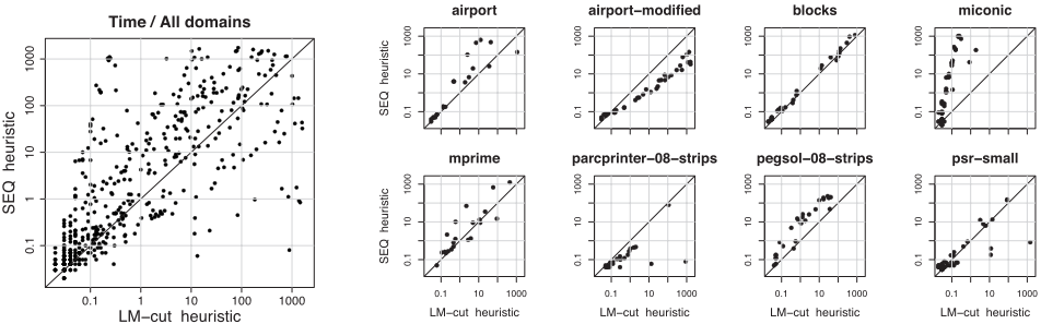
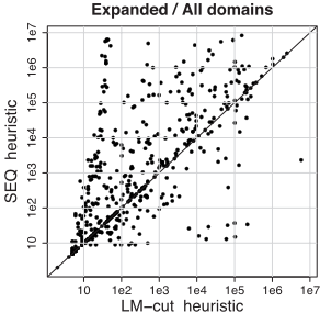
Figure 2: Comparisons of the number of expanded nodes for the SEQ and LM-cut heuristics for instances solved by both heuristics and across all domains. Points above the diagonal represent instances on which LM-cut is better, while points below it instances on which SEQ is better. Plots are in logscale.
hSEQ approximates the ILP that defines hiSEQ . In general, the LP for hSEQ does not have integral solutions, but we have observed that it does so in many problems. A known fact between ILPs and their LP relaxations is that if the matrix A that define the constraints is totally unimodular (TU), then the relaxed LP has integral solutions for any cost vector and thus solve the ILP [Korte and Vygen, 2001]. A matrix A is TU when every minor (determinant of square submatrix) has value in {-1, 0, 1}. Furthermore, it is known that the incidence matrix of any directed graph is TU. The incidence matrix of a P/T net is not the incidence matrix of the net when viewed as a directed graph, 3 yet it is similar and related to it. One can define another heuristic in terms of the ILP defined by the TU matrix of the P/T net which can then be solved exactly in polytime by just dropping the integrality constraints. However, the new heuristic is not as informative as hSEQ . We do not have yet a clear interpretation for the dual of the LP for hSEQ . Certainly it is an important issue that may shed light on the strengths and weaknesses of hSEQ and ways to improve it. We plan to study it in the near future.
We finish this discussion with a brief summary. The paper introduces a new admissible heuristic for optimal SAS+ planning that is obtained from the state equation for the Petrinet associated with the problem. The heuristic is defined in terms of an LP problem that need to be solved for each node encountered during the search. Despite the overhead of this operation, the resulting heuristic is competitive with state-ofthe-art heuristics in both number of problems solved and time to solve them.
Acknowledgements
The experiments were performed at the ORION cluster at the Universidad Pompeu Fabra, Barcelona, Spain.
@inproceedings{ijcai2013p335,
  title     = {An Admissible Heuristic for SAS+ Planning Obtained from the State Equation},
  author    = {Bonet, Blai},
  booktitle = {Proceedings of the Twenty-Third International Joint Conference on
               Artificial Intelligence, {IJCAI-13}},
  publisher = {AAAI Press / International Joint Conferences on Artificial Intelligence},
  editor    = {Francesca Rossi},
  pages     = {2268--2273},
  year      = {2013},
  month     = {8},
  url       = {https://ijcai.org/proceedings/2013/335},
}
TY - CPAPER TI - An Admissible Heuristic for SAS+ Planning Obtained from the State Equation AU - Bonet, Blai T2 - Proceedings of the Twenty-Third International Joint Conference on Artificial Intelligence, IJCAI-13 PB - AAAI Press / International Joint Conferences on Artificial Intelligence PY - 2013 SP - 2268 EP - 2273 UR - https://ijcai.org/proceedings/2013/335 ER -Copied
Machine-readable versions of this paper, for tools and AI agents:





