
Predicting Human Strategic Decisions Using Facial Expressions
Proceedings of the Twenty-Third International Joint Conference on Artificial Intelligence. Pages 2035-2040.
© 2013 International Joint Conferences on Artificial Intelligence
Abstract
People's facial expressions, whether made consciously or subconsciously, continuously reveal their state of mind. This work proposes a method for predicting people's strategic decisions based on their facial expressions. We designed a new version of the centipede game that introduces an incentive for the human participant to hide her facial expressions. We recorded on video participants who played several games of our centipede version, and concurrently logged their decisions throughout the games. The video snippet of the participants' faces prior to their decisions is represented as a fixed-size vector by estimating the covariance matrix of key facial points which change over time. This vector serves as input to a classifier that is trained to predict the participant's decision. We compare several training techniques, all of which are designed to work with the imbalanced decisions typically made by the players of the game. Furthermore, we investigate adaptation of the trained model to each player individually, while taking into account the player's facial expressions in the previous games. The results show that our method outperforms standard SVM as well as humans in predicting subjects'strategic decisions. To the best of our knowledge, this is the first study to present a methodology for predicting people's strategic decisions when there is an incentive to hide facial expressions.
- [Akbani et al., 2004] R. Akbani, S. Kwek, and N. Japkow- icz. Applying support vector machines to imbalanced datasets. Machine Learning: ECML 2004, pages 39-50, 2004.
- [Chawla et al., 2011] N. V. Chawla, K. W. Bowyer, L. O. Hall, and W. P. Kegelmeyer. SMOTE: synthetic minor- ity over-sampling technique. arXiv:1106.1813, June 2011. Journal Of Artificial Intelligence Research, Volume 16, pages 321-357, 2002.
- [Cortes and Mohri, 2004] C. Cortes and M. Mohri. AUC op- timization vs. error rate minimization. Advances in neural information processing systems, 16(16):313-320, 2004.
- [Cortes and Vapnik, 1995] C. Cortes and V. Vapnik. Support-vector networks. Machine learning, 20(3):273- 297, 1995.
- [de Melo et al., 2012] C. M. de Melo, P. Carnevale, S. Read, D. Antos, and J. Gratch. Bayesian model of the social effects of emotion in decision-making in multiagent sys- tems. In Proceedings of the 11th International Conference on Autonomous Agents and Multiagent Systems-Volume 1, pages 55-62. International Foundation for Autonomous Agents and Multiagent Systems, 2012.
- [Erev and Roth, 1998] I. Erev and A. E. Roth. Predicting how people play games: Reinforcement learning in ex- perimental games with unique, mixed strategy equilibria. American economic review, pages 848-881, 1998.
- [Kalman, 1960] R. E. Kalman. A new approach to linear fil- tering and prediction problems. Journal of basic Engineer- ing, 82(1):35-45, 1960.
- [Keshet et al., 2009] J. Keshet, D. Grangier, and S. Bengio. Discriminative keyword spotting. Speech Communication, 51(4):317-329, 2009.
- [Meijering et al., 2012] B. Meijering, H. van Rijn, N. A. Taatgen, and R. Verbrugge. What eye movements can tell about theory of mind in a strategic game. PloS one, 7(9):e45961, 2012.
- [Raiman et al., 2011] N. Raiman, H. Hung, and G. Englebi- enne. Move, and i will tell you who you are: detecting deceptive roles in low-quality data. In Proceedings of the 13th international conference on multimodal interfaces, pages 201-204, 2011.
- [Rosenthal, 1981] R. W. Rosenthal. Games of perfect in- formation, predatory pricing and the chain-store paradox. Journal of Economic Theory, 25(1):92-100, 1981.
- [Rossi et al., 2011] F. Rossi, I. Fasel, and A. G. Sanfey. In- scrutable games? facial expressions predict economic be- havior. BMC Neuroscience, 12(Suppl 1):P281, 2011.
- [Sanfey et al., 2003] A. G. Sanfey, J. K. Rilling, J. A. Aron- son, L. E. Nystrom, and J. D. Cohen. The neural basis of economic decision-making in the ultimatum game. Sci- ence, 300(5626):1755-1758, 2003.
- [Vapnik, 1998] V. N. Vapnik. Statistical Learning Theory. Wiley, 1998.
- [Veropoulos et al., 1999] K. Veropoulos, C. Campbell, and N. Cristianini. Controlling the sensitivity of support vec- tor machines. In Proceedings of the International Joint Conference on Artificial Intelligence, volume 1999, pages 55-60, 1999.
- [Yun et al., 2008] K. Yun, D. Chung, and J. Jeong. Emo- tional interactions in human decision making using eeg hyperscanning. In International Conference of Cognitive Science, 2008.
- [Yun, 2013] K. Yun. On the same wavelength: Face-to-face communication increases interpersonal neural synchro- nization. The Journal of neuroscience: the official journal of the Society for Neuroscience, 33(12):5081-5082, 2013.
References were extracted automatically from the PDF and may contain errors.
Full text extracted automatically from the PDF; figures, tables and equations may differ. The PDF is the version of record.
1 Introduction
When engaging in strategic situations where any piece of information can be crucial in order to make the best decision, people enjoy a diverse set of senses at their disposal. One of the main senses is sight, more specifically the ability to
∗These authors contributed equally to this work.
†Also affiliated with the Institute for Advanced Computer Studies at the University of Maryland.
Moshe Bitan∗
Computer Science Bar Ilan University Israel
bitanm2@macs.biu.ac.il
Sarit Kraus†
Computer Science Bar Ilan University Israel
sarit@cs.biu.ac.il
recognize emotions and facial expressions which may offer clues to intentions. A computer system that would be able to exploit this rich information would reap the benefits of a distinct advantage in a strategic situation. This paper is focused on predicting strategic decisions based on facial expressions, in those scenarios when there is a high incentive to hide them.
The strategic scenario studied in this paper is based on the centipede game [Rosenthal, 1981]. It is an extensive-form game in which two players alternately decide whether to take the larger portion of a continually increasing pot. Specifically, each player decides whether to stay (or collaborate), and then the amount in the pot increases, or to leave (or defect), and then the game ends with that player getting the larger portion of the pot while the other player gets the smaller portion. In order to introduce an incentive for the players to hide their facial expressions, we changed the game so that both players make their decisions simultaneously.
In our settings, participants are asked to play several games and are video recorded before making a decision. The video is analyzed and key facial points are extracted at each time frame in order to create a sequence of facial points. Those sequences are used as input to a classifier that is trained to predict participants' decisions. While most standard classifiers get a fix length input, the sequences of facial points are obviously of different lengths. To address this problem we represent the variable length sequences as a fixed length vector by estimating the covariance matrix of the facial points movements over time.
One of the challenges in using facial expressions for prediction is the inherent noise that image processing produces. Another challenge is the sparse number of training samples available of a specific person. An intuitive solution for the sparse data problem is to use samples from other people. However, people have different facial proportions and emotional responses for the same scenario, and there is an inevitable increase in noise. To address these challenges we used adapting filtering techniques to reduce the noise and applied normalization transformation, which positioned the nose and eyes' centroids to a fixed position in screen space. By using these techniques, noisy training samples from other people were successfully used for predicting individual strategic decisions.
Another difficulty arises from the way the human participants play this game. Game theory predicts that the first player will choose to leave in the first move and thus both players will receive a small and equal payoff. Several studies have demonstrated that this play is rarely observed [Erev and Roth, 1998]. Instead, players regularly show partial cooperation, as they choose stay for several moves before they eventually choose leave. This behavior introduces a real challenge in predicting their decisions using standard classifications tools since, statistically speaking, a classifier that constantly predicts stay results in a high classification accuracy. However, such a classification rule does not serve our goal. We address this issue by measuring performance by two types of functions: (i) the geometric mean of the recalls of both stay and leave and (ii) the area under the receiver operating characteristic (ROC) curve, and we trained our classifier to maximize those measurements.
We ran extensive experiments with 22 people and showed that, with a relatively small number of examples of a given subject, our methodology can predict both leave (the minority class) and stay (the majority class) with almost 70% accuracy, which is by far a much better prediction of what people do. To the best of our knowledge this is the first work on predicting people's strategic decisions in scenarios where they have an incentive to hide true emotions.
This paper is organized as follows. In Section 2 we present previous and relatedwork. In Section 3we present our variant of the centipede game and state its subgame perfect equilibrium. The formal problem definition is given in Section 4. Then, we describe the representation of the video signal and the learning algorithms in Section 5 and Section 6, respectively. Experimental results are presented in Section 7 and the paper is concluded in Section 8.
2 RelatedWork
Rossi et al. [2011] described a method for predicting Ultimatum game proposals' acceptance using participants' facial video recordings. Our work differs in several ways. First, in our simultaneous variant of the centipede game, participants have an incentive to hide their true emotions. Second, in the Ultimatum game the emotional response was a consequence of receiving a proposal, as opposed to the centipede where the facial expressions are precursors of a decision. Using visual information, both facial expressions and body language, has been used by Raiman et al. [2011]. The work described a method for detecting deceptive roles in multi-party conversations using audio and video clips of the body. We predict decisions that are more strategic than deceptive, and our method can be used where only facial information is available (e.g. video chat). In another work, de Melo et al. [2012] used a virtual character that was able to portray emotions when playing the iterated prisoner's dilemma. The virtual character's facial expressions were used to enhance human decision prediction. The work did not use the facial expressions of the human counterparts. Several studies used advanced imaging techniques for measuring brain activity in the Ultimatum game.
| player 2 | |||
|---|---|---|---|
| stay | leave | ||
| player 1 | stay | next | (0, mr ) |
| leave | (mr, 0) | ( mr 2 , mr 2 ) | |
Sanfey et al. [2003] used EEG measurments. The work suggested that unfair offers elicited activity in areas related to emotion. Similarly, Yun et al. [2008] and Yun [2013] suggested that face-to-face interactions induce more emotions and interpersonal neural synchronization. Finally, Meijering et al. [2012] used eye movements to distinguish between different reasoning methods. The work described a correlation between eye movement and thinking processes.
3 Repeated Simultaneous Centipede Game
We start by presenting our simultaneous version of the centipede game, which motivates the participants to hide their intentions. The game begins with a fixed amount of money in the pot (see Table 1). At each round of the game, each player has to decide either to stay or leave the game. Both players announce their decisions simultaneously. If both players choose stay, the game continues to the next round and the money in the pot is doubled. If only one of them chooses leave, this player gets all the money in the pot and the game ends. If both players choose leave, they split the money and the game ends. If both players choose stay in all rounds, the game terminates after 10 rounds and the players split the money evenly. Overall 15 games are played repeatedly by the same pair of players.
Like in the the original centipede game, a unique subgame perfect equilibrium exists where the players choose leave in the first round. Consider the following scenario where two players reach the final round of the game. Both players will choose leave; deviating and choosing stay yields a reward of zero. Formally, for the last round r, we denote mr as the cash amount at round r, and Pr as the probability that the second player will choose leave. The utility Ur of the first player is:
It is clear that Ur(leave) > Ur(stay) for any Pr > 0. Therefore, choosing leave is a dominant strategy for the last round. Consequently, each player should choose leave on the next to last round as well. Formally:
Given that mr = 2mr-1 we find that Ur-1(leave) > Ur-1(stay) for any Pr-1 > 0. Therefore, we find that choosing leave on the next to last round is a dominant strategy.
Following this reasoning backwards through the rounds, we can conclude that the dominant strategy is choosing leave on the first round. Empirical studies on the original game have shown, however, that people rarely converge to the subgame perfect equilibrium, but prefer to stay for several moves before they eventually choose leave [Erev and Roth, 1998].
4 ProblemDefinition
Recall that our goal is to predict each player's decisions based on her facial expressions. Since both players are symmetrical, we can analyze both of them in a similar way, and without loss of generality we will focus on predicting the decision of a single player.
Let us focus on round r of the game. Denote by ¯vr the video of the player's face recorded between the previous and the current decisions. The time stamp of the previous decision is referred to as the beginning of the current round. The video, ¯vr = (vr(1), . . . , vr(T)), is a sequence of T images, where vr(t) is the image at time frame t. We assume here that frame 1 denotes the beginning of the round and frame T denotes the relative frame at which the decision is made. The length T is different in each round and for each player, hence it is not fixed.
The player's decision in round r is denoted by yr ∈ Y, where Y = {stay, leave}. The classes of the set Y are stay and leave. Given an input video ¯vr at round r, our goal is to predict the player's decision ˆ yr, so it would be as close as possible to the true decision yr. Since it is hard to deal directly with variable length sequences, we map the video sequence ¯vr to a d-dimensional vector denoted xr ∈ Rd by a set of transformations, which will be described in the next section.
We define the prediction function f : Rd → R, that for a given input vector xr returns a real number, which represents the confidence of the prediction. The prediction itself is obtained by comparing the confidence to a threshold in the following way
We denote the loss function by L(y, ˆ y), which represents the severity of predicting ˆ y while the true label is y. One such loss function can be the standard 0-1 loss function which is defined as L(y, ˆ y) = δ[y ̸= ˆ y], where δ{π} is an indicator function and it equals 1 if the predicate π holds and 0 otherwise. This loss function is widely used in many classification tasks, but is not always suitable, especially when the classes are imbalanced, i.e. there are many more decisions of type stay then of type leave.
Several evaluation measures have been suggested to overcome the problem of imbalanced decisions. In this work we focus on two main evaluation measures: (i) the geometric mean of the recalls of both decision classes, denoted g-mean, and (ii) the area under the receiver operating characteristic (ROC) curve, abbreviated as AUC. In the next section we present the mapping of the video sequence to a fixed-size feature vector, and present in Section 6 the learning techniques that aim at maximizing these measures of performance from the training set of examples.
5 Representation of Facial Expressions
The facial expression representation at each round is based on a video snippet captured from the beginning of the round until the time that the player made a decision. Each captured video is of a different length and the goal of the representation is to extract the relevant information for the prediction as a fixedlength vector.
We are interested in a predefined set of points of the player's face. We assume that facial expressions can be modeled by analyzing the movements of the points and the interactions between them over time. The points are extracted after the face is aligned with a face tracker, while the noise in the tracking is removed by the Kalman filter [Kalman, 1960]. Empirically we found that the noise covariance is diagonal and we can use the one-dimensional version of the Kalman filter separately for each axis.
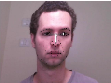
Formally, for each frame t of the video ¯vr, that is the image vr(t), we extract K facial points. Each point pk(t) ∈ N2 is a pair of absolute coordinates, where 1 ≤ k ≤ K (we omitted the round index r for the sake of readability). In our setting we used 66 points (K = 66), where the points are divided into 9 groups: left eye, right eye, left eyebrow, right eyebrow, nose, mouth, left cheek, right cheek and chin. An example of such a set of points in a single video frame can be seen in Figure 1.
We describe now the steps to transform these sequences of points into a fixed-size feature vector. In the first step, face normalization is carried out to overcome effects of different face proportions and of movements that are not related to facial expressions. The second set introduces four additional features that add information about the relative movements of the facial points over time. The last step converts the sequence into a fixed-size vector by representing the sequence by its covariance matrix.
5.1 Normalization
We describe the transformations used to normalize the facial points so as to eliminate the effects of different face proportions and general movements of the head, which we do not consider to be facial expressions. Note that some of the general head movements are considered to be facial expressions (e.g., the movement which means "yes") are handled in the next subsection. We use a multi-step transformation function on every video frame to transform the face such that the nose is centered, the eyes are fixed in the same positions, the distance between the eyes is 1 and so is the nose length.
The first transformation, M1, centers the frame around the nose center. The nose center at frame t, denoted by nc(t) , is defined as the centroid of all the points in the nose's group. The points pk(t) are translated as follows
The second transformation, M2, rotates all the points so that the eyes are aligned to the x-coordinate. Denote by re(t) and le(t) the right and left eyes' centroids at frame t, respectively. Define the vector between the eyes' centroids as eyes(t) = re(t) - le(t), and denote by ̂ eyes(t) its normalized version, ̂ eyes(t) = eyes(t)/‖eyes(t)‖. Similarly, let ec(t) be the middle point between the eyes, ec(t) = (re(t) + le(t))/2. Define the nose vector as nose(t) = ec(t) - nc(t), and the normalized vector aŝ nose(t) = nose(t)/‖nose(t)‖. The rotation is defined as

The third transformation, M3, stretches the points so that the distance between the eyes and the nose length will be 1. Namely,
5.2 Movement and Rotation
The transformed data lacks the information about the subject's movements, which can signal their intentions. To capture this information, we define four additional features for every frame t. The first and second features are defined as the difference between the position of the subject's nose's center at frame t and t - 1 along the x and y coordinates, respectively. Formally,
The third feature captures the roll rotation as the nose angle:
The fourth feature captures the yaw and pitch rotations. In our two-dimensional face projection, when subjects nod (yaw) their nose seems to shrink. When subjects turn their head from side to side (pitch), the distance between the eyes seems to change. To capture these movements we use the ratio between the nose length and the distance between the eyes:
5.3 Feature Extraction
We now describe how we mapped the sequence of T points into a fixed-length vector that is used as input for the classifier. Let zr(t) ∈ R2K+4 be the vector composed of the K normalized points pk(t) in polar coordinates and the four features, q1-4(t). Recall that this vector represents the t-th frame of video captured at round r, and there are T such vectors.
Denote by zir = (zir (1), . . . , zir (T )), for 1 ≤ i ≤ (2K+4), the vector of the i-th feature of zr(t) at round r for all 1 ≤ t ≤ T . We define the covariance matrix, Cr, as
This is a symmetric matrix of size (2K + 4)×(2K + 4). We represent this covariant matrix by the vector cr, built from its upper triangular and main diagonal. Then, we apply principal component analysis (PCA) on the vectors cr for all rounds r of all players. Finally, we generate the feature vector xr by taking the first 10 principal components of cr.
6 Learning
We turn now to describe the classification techniques used to predict the players' decisions. One of the most well known classification methods is support vector machine (SVM) [Cortes and Vapnik, 1995]. In its standard form the SVM minimizes the 0-1 loss function [Vapnik, 1998]. As discussed in Section 4, this loss function is illogical in our prediction problem, since the distribution of the classes is imbalanced.
One way to overcome this problem was proposed in [Veropoulos et al., 1999; Akbani et al., 2004], where the standard hinge loss is replaced with two hinge losses: one per each class (stay or leave), and each with his own trade-off parameter. It is known that the trade-off parameter of SVM depends on the number of examples [Vapnik, 1998], and it makes sense to use two trade-off parameters, each normalized with the actual number of examples of that class. We refer to this method as double-loss SVM.
A different technique to overcome the problem of imbalanced classes is to try to maximize the area under the ROC curve (AUC) [Cortes and Mohri, 2004; Keshet et al., 2009]. Denote by X stay the set of all input vectors for which y = stay and similarly denote by X leave the set of all input vectors for which y = leave. The ROC is a plot of the true-positive rate versus the false-positive rate of the prediction function f. The area under the ROC curve (AUC), A, is equal to the probability that the value of the function f(x) will rank a randomly chosen input xstay from X stay higher than a randomly chosen xleave fromX leave , that is
Assume that the prediction function is defined with a set of parameters θ, denoted fθ. We would like to find θ so as to maximize A,
where the expectation is taken over (x, y), drawn from a fixed but unknown distribution. We assume that we have n training examples S = {(xstay 1 , xleave 1 ), . . . , (xstay n , xleave n )}. We can replace the mean with the average of the training examples and add regularization function Ω,
INPUT: S=pairs (xstay , xleave ) from all players excluding Alice and Bob
INITIALIZE: θ trained on S
FOR r in all rounds and all games
- get Alice's video xr
- { stay if fθr-1 (xr) ≥ 0
- leave if fθr-1 (xr) < 0
- update training set: S = S ∪ {xyr r }
- update training set S with Bob's video and decision
- balance dataset S (see Section 7)
- retraining: train θ on S
Figure 2: Online adaptation.
where λ is a trade-off parameter between the loss and the regularization. Since the summand is a combinatorial quantity which is hard to minimize, a common technique in large margin classifiers like SVM is to replace it with a convex upper bound
where [π]+ = max{0, π}. In order to train such a classifier we can easily use a standard binary SVM package and introduce to it a sample version of the training set, where pairs (xstay , xleave ) are randomly drawn, as described in Section 7. We refer to this method as max AUC SVM.
Recall that according to the unique subgame perfect equilibrium, the best strategy of a player is to leave in the first round. Nevertheless, empirical evidence shows that most players prefer to choose stay. Hence, in predicting the player's decisions we would like to take advantage of her decisions in previous rounds and games. We do that in an online learning fashion in the following way.
Consider two players: Alice and Bob. Assume that we would like to predict the decisions of Alice. Let S be the set of examples of all players excluding Alice and Bob. We start by training a model from S and produce the set of parameters θ. We would like to adapt the model to the decisions made by Alice over time. At each round r the algorithm gets as input Alice's facial expression xr and makes a prediction ˆ yr. Then the algorithm gets Alice's decision for this round, yr. Alice and Bob's videos and decisions are added to S, which can be used to train subsequent models. The algorithm now trains a new model with parameters θ based on examples from all players and examples of Alice and Bob up until round r. A pseudo code of the algorithm is given in Figure 2.
7 Experimental Results
In this section we demonstrate the efficacy of our prediction method. We recruited 22 subjects, all of whom were Computer Science students. Most subjects were males (64%), with ages varying between 18-32. Subjects received an identical tutorial and needed to answer a series of basic comprehension questions about the game before being allowed to play 1 . Each participant played 15 games with another participant, and overall the players participated in 1858 rounds. The participants could see each other via a web camera, but were not able to talk. The games were recorded using the web cameras. After each game ended, the videos were processed and divided to get a separate video for each round and player. The identities of the participants were not disclosed. The reported significance in this section was measured using the Wilcoxon signed-rank test (p < 10-3 ).
We compared several training techniques that should be suitable to predict the participants' decisions: standard SVM, double-loss SVM, and max AUC SVM with and without the samples from the predicted subject's previous rounds. For brevity, we define the term history as the video snippets of the player from previous rounds and games, and define the history length as the number of those rounds. We will present the sampling technique used to create the training set for the max AUC SVM, and will show the importance of the predicted subject's history.
Table 2 summarizes the results of the training methods, where for each training technique we present the results in terms of AUC, g-mean and the recall of both the stay class and the leave class. The results are reported using crossvalidation over the subjects ("leave-one-subject-out").
More specifically, the standard SVM was trained over all training examples. We used a Gaussian kernel with parameter σ and trade-off parameter C that were tuned on a held out set. Without any enhancements, the standard SVM almost always predicted the decision as stay, resulting with an AUC of 0.535 and g-mean of 0.00.
In order to address the imbalance problem, we trained the double-loss SVM. For each subject, we trained a model using training examples from all of the other subjects, except for her opponent. Then, the resulted model was used as an initialization to train a new online model over the subject's records. We tuned the double-loss ratio, C +/C-, to be the ratio between the stay and leave frequencies (around 9). The results with a AUC of 0.574 and g-mean of 0.502 were better than standard SVM.
We also tried to address the imbalance problem using the max AUC SVM classifier. The training set used to train this classifier is composed of pairs of the form (xstay i , xleave i ), rather than the standard pairs (xi, yi) which were used in the standard SVM and the double-loss SVM. Those pairs were generated by re-sampling the minor class leave and creating a balanced number of stay and leave samples. Using this approach, there was a slight increase in the AUC with a value of 0.586, and a significant improvement of g-mean with a value of 0.564. Moreover, unlike the previous method, stay and leave accuracies were almost identical, 0.576 and 0.553 respectively.
To further improve the prediction accuracy, we added the history of the decisions of the subject in previous rounds (in the current game and the previous games), as well as her opponent's history. The same re-sampling technique described above was used to balance the history. Results with history are reported using cross-validation over the samples ("leaveone-sample-out"). With this method we got AUC of 0.583 and g-mean of 0.564. As we will see shortly, the performance constantly increases as there is more history available for training. We were able to reach a similar prediction accuracy with significantly less training samples by under-sampling the stay class of other players (instead of re-sampling the leave class), that is, the number of pairs (xstay , xleave ) is the same as the number of examples labeled as leave. The same resampling technique described above was used to balance the history. With this technique, denoted as "under-sampling" in the table we got AUC of 0.595 and g-mean of 0.572. We compare results with yet another re-sampling technique known as Synthetic Minority Over-sampling Technique (SMOTE) [Chawla et al., 2011]. This technique generates new synthetic samples via a combination of the minority class k nearest neighbors. We got almost the same performance as before with AUC of 0.600 and g-mean of 0.562.
1 The tutorial can be found at this link: http://u.cs.biu.ac.il/~sarit/ Centipede/tutorial.html
| AUC | g-mean | stay | leave | |
|---|---|---|---|---|
| standard SVM | 0.535 | 0.00 | 1.00 | 0.00 |
| double-loss SVM | 0.574 | 0.502 | 0.656 | 0.384 |
| max AUC SVM | 0.586 | 0.564 | 0.576 | 0.553 |
| + with history | 0.583 | 0.564 | 0.58 | 0.547 |
| + under sampling | 0.595 | 0.572 | 0.61 | 0.536 |
| + SMOTE | 0.600 | 0.562 | 0.596 | 0.531 |
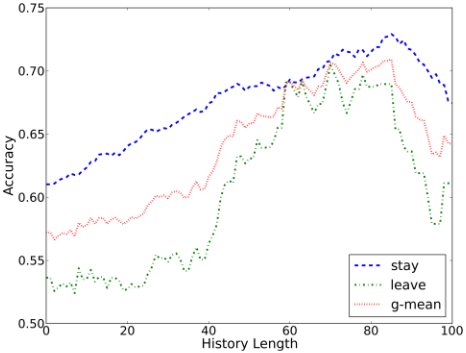
We now turn to analyze the effect of the samples from previous rounds available for training. In Figure 3 we present the accuracy of the max AUC SVM algorithm for different history lengths, where the accuracy is given in terms of g-mean, the recall of stay and the recall of leave. First, we can see that adding history generally improves accuracy. This is true until the history length of about 85; after that point the data was very sparse. Moreover, from a history length of 40 and on there is a dramatic improvement in the recall of the leave class, due to the increasing occurrence of examples of this class.
| AUC | g-mean | stay | leave | |
|---|---|---|---|---|
| standard SVM | 0.513 | 0.00 | 1.00 | 0.00 |
| double-loss SVM∗ | 0.615 | 0.414 | 0.753 | 0.228 |
| max AUC SVM∗ | 0.695 | 0.64 | 0.652 | 0.628 |
| + with history∗ | 0.726 | 0.684 | 0.67 | 0.7 |
| + under-sampling | 0.727 | 0.687 | 0.699 | 0.674 |
| + SMOTE | 0.723 | 0.687 | 0.677 | 0.698 |
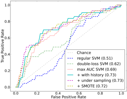
In Table 3 we present results of all training methods with a minimum history length of 70. We can see that all accuracy measurements, i.e., AUC, g-mean and recalls, improve drastically. To conclude, the ROC curves for those training methods with a minimum history length of 70 are given in Figure 4.
We conclude this section by comparing the automatic predictions to the prediction that can be made by humans. Three people, who were not any of the players, carefully observed the videos of all players' rounds and were asked to sequentially predict the players' decisions. The viewer who got the best results succeeded to predict stay samples with a recall of 0.94, but was wrong in most of leave samples with a recall of 0.24. The g-mean was 0.47, very close to the prediction of the standard SVM, and significantly worse than the g-mean of 0.687 in our classification method.
8 Conclusion
This paper presents an innovative methodology for predicting human strategic decisions using facial expressions, when there is an incentive to hide true emotions. We showed that the results are far better than chance level at around 70% recall for both leave and stay, and significantly better than the predictions made by humans. We also found that using samples from previous rounds plays important role in getting high accuracy.
We used a covariance matrix to represent the variable length video snippet as a fixed-length feature vector. It is interesting to note that we were able to make good predictions from the correlations of the position of the facial points over time, without using the positions themselves.
Acknowledgments
This work was supported in part by ERC grant #267523, the Google Inter-university center for Electronic Markets and Auctions, and ARO grants W911NF0910206 and W911NF1110344.
@inproceedings{ijcai2013p300,
  title     = {Predicting Human Strategic Decisions Using Facial Expressions},
  author    = {Peled, Noam and Bitan, Moshe and Keshet, Joseph and Kraus, Sarit},
  booktitle = {Proceedings of the Twenty-Third International Joint Conference on
               Artificial Intelligence, {IJCAI-13}},
  publisher = {AAAI Press / International Joint Conferences on Artificial Intelligence},
  editor    = {Francesca Rossi},
  pages     = {2035--2040},
  year      = {2013},
  month     = {8},
  url       = {https://ijcai.org/proceedings/2013/300},
}
TY - CPAPER TI - Predicting Human Strategic Decisions Using Facial Expressions AU - Peled, Noam AU - Bitan, Moshe AU - Keshet, Joseph AU - Kraus, Sarit T2 - Proceedings of the Twenty-Third International Joint Conference on Artificial Intelligence, IJCAI-13 PB - AAAI Press / International Joint Conferences on Artificial Intelligence PY - 2013 SP - 2035 EP - 2040 UR - https://ijcai.org/proceedings/2013/300 ER -Copied
Machine-readable versions of this paper, for tools and AI agents:





