
Robust Median Reversion Strategy for On-Line Portfolio Selection
Proceedings of the Twenty-Third International Joint Conference on Artificial Intelligence. Pages 2006-2011.
© 2013 International Joint Conferences on Artificial Intelligence
Abstract
On-line portfolio selection has been attracting increasing interests from artificial intelligence community in recent decades. Mean reversion, as one most frequent pattern in financial markets, plays an important role in some state-of-the-art strategies. Though successful in certain datasets, existing mean reversion strategies do not fully consider noises and outliers in the data, leading to estimation error and thus non-optimal portfolios, which results in poor performance in practice. To overcome the limitation, we propose to exploit the reversion phenomenon by robust $L_1$-median estimator, and design a novel on-line portfolio selection strategy named Robust Median Reversion (RMR), which makes optimal portfolios based on the improved reversion estimation. Empirical results on various real markets show that RMR can overcome the drawbacks of existing mean reversion algorithms and achieve significantly better results. Finally, RMR runs in linear time, and thus is suitable for large-scale trading applications.
- [Agarwal et al., 2006] A. Agarwal, E. Hazan, S. kale, and R.E. Schapire. Algorithms for portfolio management based on the newton method. In Proceedings of the International Conference on Machine Learning (ICML 2006), pages 9-16, 2006.
- [Aldridge, 2010] Irene Aldridge. High-Frequency Trading: A Practical Guide to Algorithmic Strategies and Trading Systems. Hoboken, NJ : Wiley, Hoboken, N.J., 2010.
- [Borodin et al., 2004] A. Borodin, R. El-Yaniv, and V. Gogan. Can we learn to beat the best stock. JAIR, 21:579-594, 2004.
- [Boyd and Vandenberghe, 2004] S. Boyd and L. Vandenberghe. Convex optimization. Cambridge University Press, New York, 2004.
- [Cover and Thomas, 1991] Thomas M. Cover and Joy A. Thomas. Elements of information theory. New York : Wiley, New York, 1991.
- T.M. Cover. Universal portfolios. Mathematical Fi- nance, 1:1-29, 1991.
- [Duchi et al., 2008] J. Duchi, S. Shalev-Shwartz, Y. Singer, and T. Chandra. Efficient projections onto the l 1-ball for learning in high dimensions. In Proceedings of the International Conference on Machine Learning (ICML 2008), 2008.
- [Gaivoronski and Stella, 2000] Alexei A. Gaivoronski and Fabio Stella. Stochastic nonstationary optimization for finding uni- versal portfolios. Annals of Operations Research, 100:165-188, 2000.
- [Grammer et al., 2006] K. Grammer, O. Dekel, J. Keshet, S. Shalev-Shwartz, and Y. Singer. Online passive-aggressive algorithms. JMLR, 7:551-585, 2006.
- [Grinold and Kahn, 1999] R. Grinold and R. Kahn. Active Portfolio Management: A Quantitative Approach for Producing Superior Returns and Controlling Risk. McGraw-Hill, New York, 1999.
- [Markowitz, 1952] H. Markowitz. Mean-variance analysis in port- folio choice and capital markets. J. Finance, 7(1):77-91, 1952.
- [Merton, 1980] R. C. Merton. On estimating the expected return on a market: An exploratory investigation. J. Financial Econ., 8:323-361, 1980.
- E. Ordentlich and T.M. Cover. On- line portfolio selection. In COLT, pages 310-313, 1996.
- [Thorp, 1971] E. O. Thorp. Portfolio choice and the kelly criterion. In Business and Economics Section of the American Statistical Association, 1971.
- [Vardi and Zhang, 2000] Yehuda Vardi and Cun Hui Zhang. The multivariate l1-median and associated data depth. PNAS, 97(4):1423-1426, 2000.
- [Weber, 1909] A. Weber. Uber den Standort der Industrien. Tub- ingen : Mohr, 1909.
- [Weiszfeld, 1937] E. Weiszfeld. Sur le point pour lequel la somme des distances de n points donnes est minimum. Tohoku Mathe- matical Journal, 43:355-386, 1937.
References were extracted automatically from the PDF and may contain errors.
Full text extracted automatically from the PDF; figures, tables and equations may differ. The PDF is the version of record.
1 Introduction
Portfolio Selection (PS) problem is concerned with determining a portfolio for allocating the wealth among a set of assets to achieve some financial objectives in the long run. There are two main mathematical models for this problem: the meanvariance model [Markowitz, 1952] and the Kelly investment [Kelly, 1956]. In general, mean-variance theory, which trades off between the expected return (mean) and risk (variance) of a portfolio, is suitable for single-period (batch) PS. While Kelly investment, which tends to maximize the expected log return, focuses on multiple-period sequential PS. Although these two theories, initially, generated little interest, they are now mainstream theories whose principles are constantly visited and re-invented. One popular research is On-line PS, which often designs algorithms following the Kelly investment because of its sequential nature, and has been actively explored in AI [Cover, 1991; Ordentlich and Cover, 1996] and machine learning communities [Agarwal et al., 2006; Borodin et al., 2004; Li and Hoi, 2012].
∗This work was partially supported by the Research Innovation Program of Shanghai MEC (13ZZ003), China PSS Foundation (201104247) and Singapore MOE tier 1 project (RG33/11).
†Corresponding Author
Some state-of-the-art on-line PS strategies [Gyorfi et al., 2006; 2008] assume that the current best performing stocks would also perform well in the next trading day, but empirical evidence [Jegadeesh., 1990] indicates that such trends may be often violated, especially in the short term. This observation leads to the strategy of buying poor performing stocks and selling those with good performance. This trading principle, known as "mean reversion", is a valid investment principle.
Recently, on-line PS [Cover, 1991; Borodin et al., 2004; Li et al., 2013; 2012a; Li and Hoi, 2012b] has exploiting the mean reversion principle. Though these mean reversion algorithms achieve encouraging results on many datasets, they perform poor on certain datasets, such as DJA dataset [Li et al., 2013; 2012a]. This is because all existing mean reversion strategies do not fully consider the noisy data and outliers, which often leads to estimation error, and thus makes the portfolio non-optimal (see [Merton, 1980]). Furthermore, the assumption of single-period prediction [Li et al., 2013; 2012a] also leads to estimation error, which thus makes the performance extremely poor [Li and Hoi, 2012b].
To address the above drawbacks, we present a new multiperiod on-line PS strategy named "Robust Median Reversion"(RMR). The basic idea is to exploit the reversion phenomenon via robust L1-median estimator [Weber, 1909; Weiszfeld, 1937; Vardi and Zhang, 2000], which explicitly estimates next price relative and is more accurate than simple mean estimator. Then we learn optimal portfolios based on the improved reversion estimation and state of the art online learning techniques.
To the best of our knowledge, RMR is the first algorithm that exploits the reversion phenomenon by robust L1-median estimator. Though simple in nature, RMR can release better estimation than existing algorithms and has been empirically validated via extensive experiments on real markets. The experimental results show that RMR significantly surpasses a number of state-of-the-art strategies in terms of long-term compound return. Moreover, it is robust to different parameter settings and it can withstand small transaction costs. Finally, RMR has linear time complexity, which is suitable for large-scale applications.
The rest of the paper is organized as follows. Section 2 formulates the on-line PS problem and Section 3 reviews some related work. Section 4 presents the proposed algorithm and Section 5 empirically evaluates its efficacy on real markets. Section 6 finally summarizes the article.
2 Problem Setting
Consider a financial market with d assets for n trading periods to be invested. On the tth period, the asset prices are represented by a close price vector pt ∈ Rd+, and each element pit represents the close price of asset i. The changes of asset prices are represented by a price relative vector xt = (x1t , . . . , xdt ) ∈ Rd+, where xjt expresses the ratio of close price to last close price of asset j at the tth period, i.e., xjt = pjt /pjt-1 . We denote xn1 = (x1, . . . , xn) as the sequence of price relative vectors for n periods.
At the beginning of the tth period, we diversify the capital among the d assets according to a portfolio vector bt = (b1t , . . . , bdt ) ∈ Rd+, where bjt represents the proportion of wealth invested in the j th asset. Typically, we assume the portfolio is self-financed and no margin/short is allowed, which means bt ∈ Δd, where Δd = {bt : bt ∈ Rd+, ∑dj=1 bjt = 1}. The investment procedure is represented by a portfolio strategy, that is, b1 = 1d 1 and following sequence of mappings bt : (Rd+)t-1 → Δd, t = 1, 2, . . . , where bt = bt(xt-1 1 ) is the portfolio used on the tth trading period given past market sequence xt-1 1 = (x1, . . . , xt-1). We denote by bn1 = (b1, . . . , bn) the strategy for n periods.
On the tth trading period, a portfolio bt achieves a portfolio period return st, that is, the wealth increases by a factor of st = bTt xt = ∑dj=1 bjt xjt . Since we reinvest and adopt price relative, the portfolio wealth would multiplicatively grow. Thus, after n trading periods, a portfolio strategy bn1 produces a portfolio cumulative wealth Sn, which increases the initial wealth by a factor of ∏nt=1 bTt xt, that is, Sn(bn1 , xn1 ) = S0 ∏nt=1 (bTt xt), where S0 is the initial wealth, which is set to 1 in this paper.
Finally, we formulate the on-line PS problem as a sequential decision task. The portfolio manager aims to design a strategy bn1 to maximize the portfolio cumulative wealth Sn. The portfolios are selected in a sequential fashion. On each period t, given the historical information, the manager learns to select a new portfolio vector bt for next price relative vector xt, where the decision criterion varies among different managers. The resulting portfolio bt is scored based on the portfolio period return of st. Such procedure repeats until the end of trading periods and the portfolio strategy is finally scored by the cumulative wealth Sn.
In the above model, we ideally assume no transaction cost, perfect market liquidity and zero impact cost. These assumptions are not trivial, which has been explained in all existing work (refer to Section 3 for detail). We will empirically analyze the effects of transaction costs in Section 5.2.
3 RelatedWork
On-line portfolio selection has been extensively explored following the principle of Kelly investment [Kelly, 1956]. One classical strategy is Constantly Rebalanced Portfolios (CRP), which keeps fixed weight on each asset for every period. Best CRP (BCRP) [Cover, 1991], the best CRP strategy over a whole market sequence, is an optimal strategy if the market is i.i.d. [Cover and Thomas, 1991]. Successive Constantly Rebalanced Portfolios (SCRP) [Gaivoronski and Stella, 2000] and Online Newton Step (ONS) [Agarwal et al., 2006] implicitly estimate next price relative via all historical price relatives with a uniform probability 1 .
Besides estimation via all historical price relatives, some strategies predict next price relatives by selecting a set of similar price relatives. Nonparametric kernel based moving window (BK ) [Gyorfi et al., 2006] measures the similarity by kernel method. Following the same framework, Nonparametric Nearest Neighbor (BNN ) [Gyorfi et al., 2008] locates the set of price relatives via nearest neighbor methods. Li et.al [2011] proposed Correlation-driven Nonparametric learning (CORN), which measures the similarity via correlation.
Moreover, another category of estimation is to predict next price relative via a single-value prediction. Exponential Gradient (EG)[Helmbold et al., 1998] estimates next price relative as last price relative. Passive Aggressive Mean Reversion (PAMR) [Li et al., 2012a] and Confidence Weighted Mean Reversion (CWMR) [Li et al., 2013] estimate next price as the inverse of last price relative, which is in essence the mean reversion principle 2 . Recently, Li and Hoi [2012b] proposed On-Line Moving Average Reversion (OLMAR), which predicts the next price relative using moving averages and explores the multi-period mean reversion.
Finally, some algorithms do not focus on estimation, either explicitly or implicitly. Universal portfolios (UP) [Cover, 1991] is the historical performance weighted average of all CRPs. Anti-Correlation (Anticor) [Borodin et al., 2004] adopts the consistency of positive lagged cross-correlation and negative autocorrelation to adjust the portfolio.
3.1 Analysis of ExistingWork
Now, let us focus on the estimation methods of existing work. In practice, a Kelly portfolio manager [Kelly, 1956; Thorp, 1971] firstly predicts ˆxt+1 in terms of k possible values ˆx1t+1 , . . . , ˆxkt+1 and their corresponding probabilities p1, . . . , pk, where each ˆxit+1 denotes one possible combination vector of individual price relative predictions. Then he/she can figure out a portfolio by maximizing the expected log return on the possible combinations,
1 SCRP and ONS's formulations are similar, while they use different techniques to solve the formulations.
2 PAMR and CWMR adopt the same estimation, while they exploit the principle via different techniques.
As different estimation methods result in different ˆxit+1 and pi and lead to different portfolio, an accurate estimation method is crucial to the success of a strategy.
Below, we focus on the algorithms PAMR, CWMR and OLMAR, which estimate next price relative via a single value prediction based on mean reversion or moving average reversion. PAMR and CWMR implicitly assume ˆx1t+1 = 1 xt with p1 = 100%, i.e., they estimate next price relative as the inverse of last price relative, which is in essence the mean reversion principle. From the price perspective [Li and Hoi, 2012b], they implicitly assume that next price ˆpt+1 will revert to last price pt-1,
where x and p are all vectors and the above operations are element-wise. Rather than ˆpt+1 = pt-1, OLMAR estimates the next price as a moving average at the end of tth period, that is, ˆpt+1 = MAt (w) = 1w ∑i=t i=t-w+1 pi where MAt (w) denotes the moving average with a w-window. Though empirically effective on most datasets, current estimation methods in PAMR/CWMR and OLMAR cause two potential problems. Firstly, the single-period mean reversion assumption of PAMR and CWMR may not be satisfied in the real world. One real example [Li et al., 2012a] is DJA dataset [Borodin et al., 2004], on which PAMR performs the worst among the state of the art. Secondly, all three algorithms suffer from the frequently fluctuating raw prices,which often contain a lot of noises and outliers. The two drawbacks thus motivate the proposed method.
4 Robust Median Reversion
4.1 Motivation
Empirical results [Li et al., 2013; 2012a] show that if asset price follows the normal distribution, the mean of historical prices may better explain the markets. OLMAR, which estimates next price via moving average, also achieves good results on most datasets. However, due to noises and outliers in the data, the price distribution often has longtail, thus previous estimation methods are sub-optimal on the real markets.
To illustrate the drawbacks of mean and moving average, let us see a toy example. The toy market consists of one volatile stock, and ti(i ≥ 0) denotes the period that requires estimation. Several sequences of market prices are listed in Table 1. A0,A1 are single-period price sequences and their prices change by sequent factor of 2, 12 , 2, 12 , . . .. For example, let Pti be the price of the ith period, then Pt1 =Pt0 ×2=1×2=2, Pt2 =Pt1 × 12 =2× 12 =1, Pt3 =Pt2 ×2 = 1×2=2, . . .. B0, B1 are two-period price sequences and their prices change by sequent factor of 2, 2, 12 , 12 , 2, 2, . . .. C0, C1 are the three-period price sequences, and the price changes by sequent factor of 2, 2, 2, 12 , 12 , 12 , 2, 2, 2, . . .. Moreover, A0,B0,C0 are exact price sequences, while A1,B1,C1 are the sequences contaminated by a outlier of 10. "?" denotes the price to be estimated and "Acc" is the accurate price. The estimated prices clear show that the next prices estimated by PAMR/CWMA and OLMAR are far away from the accurate values, which thus leads to inaccurate price relatives and suboptimal portfolios. Contrarily, the proposed methods release much better estimations (the calculation will be detailed later) and subsequent better portfolios. Note that although the toy example is on a single asset, such estimation goodness can be easily extended to the scenario of multiple assets.
| Price:t0 → t1 → . . . | Acc | PAMR/ CWMR | OLMAR | RMR |
| A0 : 1, 2, 1, 2, ? A1 : 1, 2, (10), 2, ? | 1 1 | 1 10 | 1.5 3.75 | 1.5 2 |
|---|---|---|---|---|
| B0 : 1, 2, 4, 2, ? | 1 | 4 | 2.25 | 2 |
| B1 : 1, 2, (10), 2, ? | 1 | 10 | 3.75 | 2 |
| C0 : 1, 2, 4, 8, 4, 2, ? | 1 | 4 | 3.5 | 3 |
| C1 : 1, 2, 4, 8, (10), 2, ? | 1 | 10 | 4.5 | 3 |
To better exploit (multiple period) reversion property, we proposed a new type of algorithms for on-line PS, named "Robust Median Reversion" (RMR). The essential idea is to exploit multiple period reversion via robust L1-median estimator [Weber, 1909; Weiszfeld, 1937; Vardi and Zhang, 2000] and power online machine learning. Rather than ˆpt+1 = pt-1 or ˆpt+1 = MAt(w), RMR estimates next price by robust L1-median estimator at the end of tth period, that is, ˆpt+1 = L1medt+1(w) = μ, where w is the window size, μ denotes the value in L1-median estimator that satisfied the Optimization Problem 1 below (see section 4.2). Then the expected price relative with L1-median estimator is
Without detailing the calculation, we list the estimated next price of RMR in different toy markets in Table 1. Clearly, for the multiple period price sequences B0,B1 and C0,C1, RMR estimator is much closer to the Accurate estimator than PAMR/CWMR, showing that RMR method can deal with multiple period price sequence. For the contaminated price sequences A1, B1, C1, RMR is also closer to the Accurate estimator than OLMAR and PAMR/CWMR estimators, which shows that RMR is a robust method.
Moreover, L1-median estimator is much better than mean estimators statistically. In fact, the L1-median has an attractive statistical properties, that is, its breakdown point is 0.5 [Lopuhaa and Rousseeuw, 1991], i.e., only if more than 50% of the data points are contaminated, the L1-median can take values beyond all bounds. Note that breakdown point, the proportion of incorrect observations an estimator can handle, is a statistical metric of robustness. The higher the breakdown point of an estimator is, the more robust it is. However, the breakdown point of mean is 0, which means that the mean estimator is sensitive to the noisy data and outliers.
Based on the expected price relative vector in Eq. (1), RMR further adopts the idea of an effective online learning algorithm, that is, Passive Aggressive (PA) [Grammer et al., 2006] learning, to exploit median reversion. Generally proposed for classification, PA passively keeps the previous solutions if the classification is correct, while aggressively approaches a new solution if the classification is incorrect. After formulating the proposed RMR optimization, we solve its closed form update and design the proposed algorithm.
4.2 Formulation
The proposed formulation, RMR, is to exploit median reversion via robust L1-estimator and PA online learning. The basic idea is to obtain next price relative ˆxt+1 via multivariate L1-median, and then maximize the expected return b · ˆxt+1 while keeping last portfolio information via regularization.
To estimate the next price relative ˆxt+1, we calculate the multivariate L1-median of historical prices. In statistics, the L1-median (also named spatial median) of a k-historical price window, μ, is the solution of following optimization,
Optimization problem 1: L1-median
where ‖·‖ denotes the Euclidean norm. In a word, L1-median is the point with minimal sum of Euclidean distances to the k given price data points. This problem is formulated in an even more general form by Weber [Weber, 1909] (FermatWeber problem), as he refers to location issues in industrial contexts. If the data points are not collinear, the solution to problem (2) is unique [Weiszfeld, 1937].
After obtaining the L1-median estimator of price, we can calculate next price relative ˆxt+1 by Eq. (1). Based on the obtained price relative ˆxt+1, we can select next portfolio via PA online learning technique. Thus, following the similar idea PAMR and OLMAR [Li et al., 2012a; Li and Hoi, 2012b], we can formulate the following optimization,
Optimization problem 2: RMR
The above formulation attempts to find an optimal portfolio by minimizing the deviation from last portfolio bt under the condition of b · ˆxt+1 ≥ ε. Such formulation explicitly reflects the reversion idea underlying the proposed RMR. In fact, ˆxt+1 is the price relative estimated via L1-median estimator, while the constraint b· ˆxt+1 ≥ ε means that next price will revert to the L1-median.
4.3 Algorithm
To obtain the L1-median of historical prices, we apply the Modified Weiszfeld Algorithm [Vardi and Zhang, 2000], which converges monotonically to the L1-median. The solution of L1-median described in Eq. (2) is illustrated below.
Proposition 1 The solution of L1-median optimization problem 1 is calculated through iteration, and the iteration process is described as:
where
,
In general, we often practically set the convergence criterion during the iteration. Here, once the constraint of ‖μι-1 -μι‖1 ≤ τ‖μι‖1 is satisfied, we terminate the iteration. Note that τ represents a toleration level.
We now obtain the final portfolio selection formula by solving the Optimization problem 2, which is convex and thus straightforward to solve via the Lagrange multiplier method [Boyd and Vandenberghe, 2004].
Proposition 2 The solution of the Optimization problem 2 without considering the non-negativity constraint is
where xt+1 = 1d (1· ˆxt+1) denotes the average predicted price relative and αt+1 is the Lagrangian multiplier calculated as,
Note that it is possible that the resulting portfolio in Proposition 2 goes out of the simplex domain since we do not consider the non-negativity constraint. Thus, to ensure that the portfolio is non-negative, we finally project the above portfolio to the simplex domain [Duchi et al., 2008].
To this end, we can design the proposed algorithms based on the above Propositions. The estimated process of price relative ˆxt+1, mainly based on Proposition 1, is illustrated in Algorithm 1. The proposed RMR procedure, which is designed up on Proposition 2, is shown in Algorithm 2. Finally, Algorithm 3 presents the on-line portfolio selection following the problem setting in Section 2.
4.4 Analysis
It is widely known that computational time is important to certain trading environments, such as high frequency trading [Aldridge, 2010], which occurs in fractions of a second. RMR's time complexity is linear with respect to d and n, where n is much larger than d. In the RMR implementation, the max number of loop (Line 6 in Algorithm 1) can be implemented in O(m). Thus, Algorithm 1 take O(m) time
Algorithm 1 L1 median (pt, pt-1, . . . , pt-w+1, m, τ )
- 1: Input: data pt, pt-1, . . . , pt-w+1; iteration maximum m; toleration level τ
- 2: Output: estimated ˆxt+1
- 3: Procedure:
- 4: Initialize μ1 = median(pt, pt-1, . . . , pt-w+1).
- 5: for i = 2 to m do
- 6: μi = T (μi-1)
- 7: if ‖μi-1 -μi‖1 ≤ τ‖μi‖1 then
- 8: break
- 9: end if
- 10: end for
- 11: ˆpt+1 = μi
- 12: ˆxt+1 = ˆpt+1/pt
Algorithm 2 RMR(ϵ, ˆxt+1, bt)
- 1: Input: reversion threshold ϵ > 1; predicted next price relative vector ˆxt+1; current portfolio bt;
- 2: Output: next portfolio bt+1
- 3: Procedure:
- 4: Calculate the following variable:
- 5: Update the portfolio:
- 6: Normalize bt+1: bt+1 = argminb∈Δd ‖b-bt+1‖2
per period. Moreover, Algorithm 2 takes O(d) per period. In total, the whole time complexity is O(dn) + O(mn). Table 2 compares the time complexity of RMR with that of existing strategies. Clearly, the proposed RMR algorithm takes no more time than any others.
| Methods | Time Complexity | Methods | Time Complexity |
|---|---|---|---|
| UP EG PAMR/CWMR /OLMAR | O (nd )/O (d7 n8 ) O (dn) O(dn) | ONS Anticor BK/BNN /CORN | O (d3 n) O (N 3 d2 n) O (N 2 dn2 ) +O (Ndn2 ) |
| RMR | O (dn) + O (mn) |
5 Experiments
5.1 Datasets
We test the portfolio strategies on four public datasets from real markets 3 , which are summarized in Table 3.
Pioneered by Cover [1991], NYSE(O) is one benchmark dataset, which consists of 36 stocks from the New York Stock
3 All datasets and their compositions can be downloaded from http://www.cais.ntu.edu.sg/ chhoi/olps/datasets.html.
Algorithm 3 Portfolio selection with RMR
- 1: Input: reversion threshold ϵ > 1; iteration maximumm; window size w ≥ 2; toleration level τ; market sequence xn1
- 2: Output: Sn: Cumulative wealth after nth periods
- 3: Procedure:
- 4: Initialization: b1 = 1d 1, S0 = 1, p0 = 1
- 5: for i = 1 to n do
- 6: pi = xi · pi-1
- 7: end for
- 8: for t = 1, 2, . . . , n do
- 9: Receive stock price: xt
- 10: Update cumulative return: St = St-1 × (bt · xt)
- 11: Predict next price relative vector:
- 12: Update the portfolio:
13: end for
Exchange. Extended from NYSE(O), NYSE(N) [Li et al., 2013] contains 23 stocks. The dataset DJA is collected by Borodin et al. [2004] and consists of DowJones 30 composite stocks. The final dataset MSCI is a collection of 25 global equity indices that are the constituents of MSCI World Index.
| DATA SET | REGION | TIME FRAME | #DAYS | #ASSETS |
|---|---|---|---|---|
| NYSE(O) | US | 3/7/1962-31/12/1984 | 5651 | 36 |
| NYSE(N) | US | 1/1/1985-30/6/2010 | 6431 | 23 |
| DJA | US | 1/1/2001-14/1/2003 | 507 | 30 |
| MSCI | GLOBAL | 1/4/2006-31/3/2010 | 1043 | 24 |
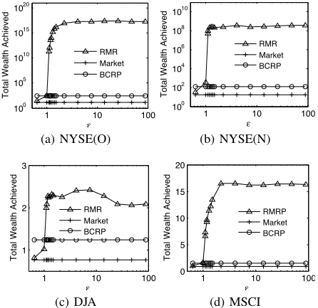
RMR has two possible parameters, i.e., w and ε, which can be tuned to obtain optimal results. To consistently compare different methods, we empirically set the parameter w=5, ε=5 and m = 200 on all settings. Our experiments on parameter sensitivity clearly show that our empirical choice is not the best in hindsight.
5.2 Experimental Results
Cumulative wealth
Table 4 summarizes the cumulative wealth achieved by various methods. From the figure, we can see that RMR outperform the state of the art on NYSE(O), NYSE(N) and DJA. On MSCI, RMR beats most existing algorithms, including OLMAR. Besides, the maximum cumulative wealth is even better than RMR, showing the potential of the proposed method. Finally, Table 5 shows some statistics [Grinold and Kahn, 1999] of RMR. From the results, we can observe small pvalues, which means that RMR's excellent performance is not due to luck but owed to the strategy principle.
Parameter sensitivity
Firstly, we examine the effect of sensitivity parameter ϵ on cumulative wealth, in Figure 1. The cumulative wealth sharply grows as ϵ increases and then flattens when ϵ crosses a threshold. Secondly, we examine the effect of window size w, in Figure 2. The cumulative wealth decreases with increasing w. Obviously, RMR's performance with a large number of ϵ and w is better than the two benchmarks. All above observations clearly show that RMR is robust w.r.t. different parameters and it is convenient to choose satisfying parameters.
| Methods | NYSE(O) | NYSE(N) | DJA | MSCI |
|---|---|---|---|---|
| Market | 14.50 | 18.06 | 0.76 | 0.91 |
| Best-stock | 54.14 | 83.51 | 1.19 | 1.50 |
| BCRP | 250.60 | 120.32 | 1.24 | 1.51 |
| UP | 26.68 | 31.49 | 0.81 | 0.92 |
| EG | 27.09 | 31.00 | 0.81 | 0.93 |
| ONS | 109.91 | 21.59 | 1.53 | 0.86 |
| Bk | 1.08E+09 | 4.64E+03 | 0.68 | 2.64 |
| BNN | 3.35E+11 | 6.80E+04 | 0.88 | 13.47 |
| CORN | 1.48E+13 | 5.37E+05 | 0.84 | 26.19 |
| Anticor | 2.41E+08 | 6.21E+06 | 2.29 | 3.22 |
| PAMR | 5.14E+15 | 1.25E+06 | 0.68 | 15.23 |
| CWMR | 6.49E+15 | 1.41E+06 | 0.68 | 17.28 |
| OLMAR | 4.04E+16 | 2.24E+08 | 2.05 | 16.33 |
| RMR | 1.64E+17 | 3.25E+08 | 2.67 | 16.76 |
| RMR(max) | 2.81E+17 | 4.73E+08 | 3.47 | 19.07 |
| Stat. | NYSE(O) | NYSE(N) | DJA | MSCI |
|---|---|---|---|---|
| Size | 5651 | 6431 | 507 | 1043 |
| MER(RMR) | 0.0077 | 0.0036 | 0.0024 | 0.0030 |
| MER(Market) | 0.0005 | 0.0005 | -0.0004 | 0.0000 |
| α | 0.0071 | 0.0031 | 0.0030 | 0.0030 |
| β | 1.2718 | 1.1628 | 1.2427 | 1.1885 |
| t-statistics | 15.7325 | 7.4222 | 2.5217 | 5.8380 |
| p-value | 0.0000 | 0.0000 | 0.0060 | 0.0000 |
Transaction costs
In practice, transaction cost is an important and unavoidable issue that should be addressed. We thus test the effect of proportional transaction cost when the transaction cost rate γ varies from 0 to 1%. We also plot the results achieved by two benchmarkes of BCRP and Market and the cumulative wealth achieved by PAMR[Li et al., 2012a], OLMAR[Li and Hoi, 2012b]. From Figure 3, we can observe that RMR can withstand reasonable transaction cost rates, and can beat the two benchmarks and PAMR, OLMAR.
6 Conclusions
In this paper, we propose a novel multiple period on-line portfolio selection strategy named "robust median reversion" (RMR), which exploits the reversion phenomenon of stock prices by robust L1-median estimator and online learning technologies. The proposed approach can solve the problems of the state of the art caused by the noisy data and outliers as well as the single-period mean reversion. Extensive experiments on real markets show that the proposed RMR can achieve satisfying performance. In future, we will study other robust estimation methods and adaptive parameter methods and theoretically analyze the median reversion.
@inproceedings{ijcai2013p296,
  title     = {Robust Median Reversion Strategy for On-Line Portfolio Selection},
  author    = {Huang, Dingjiang and Zhou, Junlong and Li, Bin and Hoi, Steven C. H. and Zhou, Shuigeng},
  booktitle = {Proceedings of the Twenty-Third International Joint Conference on
               Artificial Intelligence, {IJCAI-13}},
  publisher = {AAAI Press / International Joint Conferences on Artificial Intelligence},
  editor    = {Francesca Rossi},
  pages     = {2006--2011},
  year      = {2013},
  month     = {8},
  url       = {https://ijcai.org/proceedings/2013/296},
}
TY - CPAPER TI - Robust Median Reversion Strategy for On-Line Portfolio Selection AU - Huang, Dingjiang AU - Zhou, Junlong AU - Li, Bin AU - Hoi, Steven C. H. AU - Zhou, Shuigeng T2 - Proceedings of the Twenty-Third International Joint Conference on Artificial Intelligence, IJCAI-13 PB - AAAI Press / International Joint Conferences on Artificial Intelligence PY - 2013 SP - 2006 EP - 2011 UR - https://ijcai.org/proceedings/2013/296 ER -Copied
Machine-readable versions of this paper, for tools and AI agents:





