
Multi Class Learning with Individual Sparsity
Proceedings of the Twenty-Third International Joint Conference on Artificial Intelligence. Pages 1729-1734.
© 2013 International Joint Conferences on Artificial Intelligence
Abstract
Multi class problems are everywhere. Given an input the goal is to predict one of a few possible classes. Most previous work reduced learning to minimizing the empirical loss over some training set and an additional regularization term, prompting simple models or some other prior knowledge. Many learning regularizations promote sparsity, that is, small models or small number of features, as performed in group LASSO. Yet, such models do not always represent the classes well. In some problems, for each class, there is a small set of features that represents it well, yet the union of these sets is not small. We propose to use other regularizations that promote this type of sparsity, analyze the generalization property of such formulations, and show empirically that indeed, these regularizations not only perform well, but also promote such sparsity structure.
- [Bach et al., 2011] Francis Bach, Rodolphe Jenatton, Julien Mairal, and Guillaume Obozinski. Convex optimization with sparsity- inducing norms. In Optimization for Machine Learning. MIT Press, 2011.
- [Bakin, 1999] Sergey Bakin. Adaptive regression and model selec- tion in data mining problems, 1999. Thesis (Ph.D.)-Australian National University, 1999.
- [Bartlett and Mendelson, 2003] Peter L. Bartlett and Shahar Mendelson. Rademacher and gaussian complexities: risk bounds and structural results. J. Mach. Learn. Res., 3:463-482, March 2003.
- [Benedek and Panzone, 1961] A Benedek and Panzone. R.: The space lp, with mixed norm. Duke Math. J, (28):301-324, 1961.
- [Boser et al., 1992] Bernhard E. Boser, Isabelle M. Guyon, and Vladimir N. Vapnik. A training algorithm for optimal margin classifiers. In Proceedings of the fifth annual workshop on Com- putational learning theory, COLT '92, pages 144-152, 1992.
- [Bradley and Bagnell, 2009] David Bradley and J. Andrew (Drew) Bagnell. Convex coding. Technical Report CMU-RI-TR-09-22, Robotics Institute, Pittsburgh, PA, May 2009.
- [Combettes and Pesquet, 2011] Patrick Combettes and Jean- Christophe Pesquet. Proximal splitting methods in signal processing. In H.H. Bauschke, R.S. Burachik, P.L. Combettes, V. Elser, D.R. Luke, and H. Wolkowicz, editors, Fixed-Point Algorithms for Inverse Problems in Science and Engineering, pages 185-212. Springer, 2011.
- [Cortes and Vapnik, 1995] Corinna Cortes and Vladimir Vapnik. Support-vector networks. In Machine Learning, volume 20, pages 273-297, 1995.
- [Crammer and Singer, 2001] Koby Crammer and Yoram Singer. On the algorithmic implementation of multiclass kernel-based vector machines. Journal of Machine Learning Research, 2:265- 292, December 2001.
- [Crammer et al., 2009] Koby Crammer, Mark Dredze, and Alex Kulesza. Multi-class confidence weighted algorithms. In EMNLP, pages 496-504, 2009.
- [Duchi and Singer, 2009a] John Duchi and Yoram Singer. Boosting with structural sparsity. In ICML, ICML '09, 2009.
- [Duchi and Singer, 2009b] John Duchi and Yoram Singer. Efficient learning using forward-backward splitting. In NIPS, pages 495- 503, 2009.
- [Fornasier and Rauhut, 2008] Massimo Fornasier and Holger Rauhut. Recovery algorithms for vector-valued data with joint sparsity constraints. SIAM Journal on Numerical Analysis, 46(2):577-613, 2008.
- [Hoerl and Kennard, 1970] A E Hoerl and R W Kennard. Ridge regression: Biased estimation for nonorthogonal problems. Tech- nometrics, (12):55-67, 1970.
- [Hoerl, 1962] A E Hoerl. Application of ridge analysis to regres- sion problems. Chemical Engineering Progress, 58(3):54-59, 1962.
- [Kowalski and Torrésani, 2008] Matthieu Kowalski and Bruno Torrésani. Sparsity and persistence: mixed norms provide sim- ple signal models with dependent coefficients. Signal Image and Video Processing, 3(3):251-264, 2008.
- [Kowalski et al., 2009] Matthieu Kowalski, Marie Szafranski, and Liva Ralaivola. Multiple indefinite kernel learning with mixed norm regularization. In Proceedings of the 26th Annual Interna- tional Conference on Machine Learning, ICML '09, pages 545- 552, 2009.
- [Kowalski, 2009] Matthieu Kowalski. Sparse regression using mixed norms. Applied and Computational Harmonic Analysis, 27(3):303 -324, 2009.
- [Lee et al., 2004] Yoonkyung Lee, Yi Lin, and Grace Wahba. Mul- ticategory support vector machines, theory, and application to the classification of microarray data and satellite radiance data. Jour- nal of the American Statistical Association, 99:67-81, 2004.
- [Mairal et al., 2010] Julien Mairal, Rodolphe Jenatton, Guillaume Obozinski, and Francis Bach. Network flow algorithms for struc- tured sparsity. In Advances in Neural Information Processing Systems 23, pages 1558-1566. 2010.
- [Massart, 2000] Pascal Massart. Some Applications of Concentra- tion Inequalities to Statistics. Annales de la Faculté des Sciences de Toulouse, IX(2):245-303, 2000.
- [Moreau, 1962] J Moreau. Fonctions convexes duales et points proximaux dans un espace hilbertien. CR Acad. Sci. Paris Sér. A Math, (255), 1962.
- [Mukherjee et al., 2002] Sayan Mukherjee, Ryan Rifkin, and Tomaso Poggio. Regression and classification with regulariza- tion, 2002.
- [Szafranski et al., 2008] Marie Szafranski, Yves Grandvalet, and Pierre Morizet-Mahoudeaux. Hierarchical penalization. In Advances in Neural Information Processing Systems 20 (NIPS 2007), 2008.
- [Teschke and Ramlau, 2007] Gerd Teschke and Ronny Ramlau. An iterative algorithm for nonlinear inverse problems with joint spar- sity constraints in vector-valued regimes and an application to color image inpainting. Inverse Problems, 23(5):1851, 2007.
- [Tibshirani, 1996] R Tibshirani. Regression shrinkage and selection via the lasso. Journal of the Royal Statistical Society. Series B (Methodological, (58), 1996.
- [Tikhonov and Arsenin, 1977] A N Tikhonov and V Y Arsenin. So- lutions of ill posed problems, 1977.
- [Weston and Watkins, 1998] J Weston and C Watkins. Multi-class support vector machines. Pattern Recognition, (CSD-TR-98- 04):0-9, 1998.
- [Xu et al., 2009] H Xu, C Caramanis, and S Mannor. Robustness and regularization of support vector machines. Journal of Ma- chine Learning Research, (10):1485-1510, 2009.
- [Yuan and Lin, 2006] Ming Yuan and Yi Lin. Model selection and estimation in regression with grouped variables. Journal of the Royal Statistical Society, Series B, 68:49-67, 2006.
- [Zhao et al., 2009] Peng Zhao, Guilherme Rocha, and Bin Yu. The composite absolute penalties family for grouped and hierarchical variable selection. ANNALS OF STATISTICS, 37:3468, 2009.
References were extracted automatically from the PDF and may contain errors.
Full text extracted automatically from the PDF; figures, tables and equations may differ. The PDF is the version of record.
1 Introduction
Regularization is a highly-used and understood task in supervised learning. Given data-samples, called training data, modern algorithms not only seek for a model that performs well on the training data, but also require that the model would be simple in some sense, where simplicity is measured via some regularization function. Regularization is widely used as a mechanism to prevent overfitting or impose prior knowledge of a structure on a model. Learning binary prediction problems or regression of real numbers is studied for over half a century, with a lot of work focusing in linear models. Given an input x ∈ ℜd , its inner product with some vector ω ∈ ℜd is used to make a prediction, f(ω⊤x). In many cases regularization is defined to be some norm of that vector, ‖ω‖.
Among others, SVM [Boser et al., 1992; Cortes and Vapnik, 1995] can be represented as such classification problem with ℓ2 norm [Mukherjee et al., 2002]. For regression, Ridge Regression [Hoerl, 1962; Hoerl and Kennard, 1970; Tikhonov and Arsenin, 1977] (ℓ2 norm) and LASSO [Tibshirani, 1996] (ℓ1 norm) are popular.
In more complex problems, such as multi class categorization, in which given an input x the algorithm is required to output one of c possible classes, matrix models ω ∈ ℜd×c are used. Here, linear models prediction is performed by first computing the inner product of the input with each column of the matrix, and then processing the resulting c scalars, f(ω⊤ 1 x, ..., ω⊤ c x). In multi class problems we have f(a1, ..., ac) = argmaxs as. Natural extensions for norm regularization from vector to matrices are entrywise norms, such as the Frobenius norm: √∑s ∑t |ωt,s|2 , used in multi class SVMs [Weston and Watkins, 1998; Crammer and Singer, 2001; Lee et al., 2004].
Alternatively a mixed norm can be used. The most common such usage is group LASSO [Yuan and Lin, 2006; Bakin, 1999] which uses the ℓ2,1 mixed norm as a mechanism for selecting a group of variables. That is, the regularization promotes choosing a small sub-set of the features (rows), and then any feature from this subset can be used. However, if we seek sparser models, then the ℓ1,1 (which is the vector ℓ1 norm in the mixed norm representation) is often used, as a convex relaxation of counting the number of non-zero elements.
We argue that for many situations these two norms are not capturing our requirements frommodels. Though it is reasonable to believe that many features are redundant, this redundancy might be different among classes. For example color pattern may be very informative for zebras, but less informative for horses, dogs, cats or chameleons which may have a variety of color patterns, and thus ℓ2,1 may not be the right choice. Additionally, the global sparsity prompted by ℓ1,1 may generate models that are very sparse for some classes, and dense for others. This may happen if the data is far from being balanced, as there are few examples of one class, and many of another classes.
In this work we propose to use another principle for regularization. Instead of forcing a small number of features (ℓ2,1) or a small model altogether (ℓ1,1), we propose to promote models, in which for each class (independently) there would be a small number of relevant features. Such regularization would generate small, that is sparse, models, yet would not "favor" certain classes. We formulate learning with such regularization in the next section and provide robustness analysis and generalization bound for this, and in fact, for all mixed norms. Specifically, we show that our regularization is equivalent to an algorithmwhich is robust to a feature noise that is different per class, yet worst classes' noise is not too large.
We also report results with 14 text classification problems, with a large range in size, number of classes and dimensions. We show that our proposed regularization attains higher F1 scores than any other mixed norm regularization we tried, yet results in sparser models. One explanation for that difference is that our algorithm attains higher recall values (over classes) paying in precision. This demonstrates exactly the point that the obtained models are not too-sparse for some classes, as models learned with ℓ1,1 regularization may be (when some classes contain very few non-zero model terms, they may never be predicted).
Relatedwork: Most workwithmixed norm regularization focussed on ℓ2,1 and ℓ∞,1 norms [Duchi and Singer, 2009b; 2009a; Bradley and Bagnell, 2009; Zhao et al., 2009; Mairal et al., 2010]. A work on mixed norm regularization including ℓ1,2 was proposed for signal estimation [Kowalski, 2009; Kowalski and Torr´esani, 2008] and kernel learning for binary classification [Kowalski et al., 2009]. In a work on hierarchical penalization [Szafranski et al., 2008] a ℓ43 ,1 norm was derived and used. The ℓp,1 norm regularization was also used in other contexts [Fornasier and Rauhut, 2008; Teschke and Ramlau, 2007].
Notation: Given a matrix A, its mixed norm, ℓp,q;r, is defined by computing the p norm of each column (or row) of A, and then computing the q norm of the result. The order of the summation (columns or rows first) is defined by r ∈ {1, 2}. We define a mixed norm where we either first sum over rows (r = 1) or over columns (r = 2),
An early work on mixed norms spaces was done by Benedek and Panzone at 1961 [Benedek and Panzone, 1961].
2 Individual Variable Selection
Group selection, promoted by group LASSO and other mixed norms of the form ℓp,1, assume that one group of variables have good descriptive qualities for the entire problem. Specifically, for feature selection in multi class, the assumption is that a subset of the features is globally able to describe well all the classes. That is, a small set is sought that would work well across all classes. We take a different route and assume that for each class there is a small number of features that describe it well. However, we do not assume that this set overlaps other classes' sets, and also, we do not want to have too small number of features for some classes. This intuition leads to the following regularization, ∑i (zero norm of column i)2 . That is, we compute the number of non-zero elements per class and then take the Euclidean norm of this vector of counts. The Euclidean norm is used, as we want to demote classes for which there are many non-zero elements compared with others. As performed in other contexts, we replace the zero norm with the unit norm, which is convex and continuous, and obtain the following relaxation,
Thus, given a training set (xi, yi) where xi ∈ ℜd and yi ∈ {1, ..., c}, we propose to learn by minimizing the following problem,
where L(ω, (xi, yi)) is some multi class loss, such as the multi class log loss (with a curvature parameter ν),
Previous work with ℓ1,2 regularization included signal reconstruction [Kowalski, 2009; Kowalski and Torr´esani, 2008] and binary classification with multiple kernels [Kowalski et al., 2009]. To the best of our knowledge no work has used ℓ1,2 regularization for multi class problems.
3 Analysis
We now provide an analysis for learning with mixed-norm matrices. First we state an equivalence to robustness over a certain noise, and then a generalization bound based on Gaussian complexity analysis. In both cases we build on previous tools, and modify them to our setting. We emphasize that it is not a direct application, but a non-trivial derivation is needed.
The properties we show in this chapter demonstrate theoretical guarantees according to a prior knowledge. This prior knowledge may guide us to choose our proposed ℓ1,2;2 regularization. We extend the equivalence of binary SVM to robust optimization [Xu et al., 2009] to a multi class setting. We also state generalization bounds for ℓ1,2;2 regularization, using Gaussian complexity.
3.1 Equivalence to noise robustness
Robustness to noise is one of regularization's main goals. Recently Xu et al. [Xu et al., 2009] showed, that with some limitations, regularization for binary classification using hinge loss, is equivalent to robust optimization. We extend this notion to the multi class setting by showing an equivalence of mixed norm regularization and robustness to noise for the sum of hinges loss function.
One approach we tried was to reduce multi class learning into a binary classification problem with c-times more examples. Applying the result of Xu et al. [Xu et al., 2009] on the new problem, provided us a robustness equivalence only to ℓp,1;2 mixed norms.
We thus re-derived this equivalence from scratch. Following the outline of Xu et al. [Xu et al., 2009] we proved the following result (here yi ∈ {-1, 1}c ).
Theorem 1 Given a set of examples {xi, yi }ni=1 , non separable for each class s = 1, ..., c (for each class s = 1, ..., c and every ωs ∈ ℜd , there is an example j(s) such that: yj(s),s(ω⊤s xj(s)) < 0, where yj(s),s is the s term of yj(s) ), and the two sets,
and
for some p∗, q∗ ≥ 1, the following two optimization problems are equivalent:
where 〈A,B〉 = Tr(A⊤B) is the matrix (Frobenius) inner product.
The proof is omitted due to lack of space. When a norm of the perturbation is bounded, the regularization term is similar to the definition of the dual norm (multiplied by the bound value). This means that ℓp∗,q∗ is the dual norm of some ℓp,q norm, where 1p + 1 p∗ = 1q + 1 q∗ = 1 [Bradley and Bagnell, 2009]. Thus, we get the regularization term:
According to Eq. (3), the correspondence between the regularization tradeoff parameter λ and the noise bound M is λ = M. In other words, λ may be used to estimate the noise bound M (= λ) and vice versa. For example, if we know that ∑ni=1 ‖δi‖∞,2;2 ≤ M, then ℓ1,2;2 would be the best regularization. In this type of noise, for each class the noise may be different, yet it does not get too high, as the norm of largest classes' noise, summed over examples should not be too large.
3.2 Generalization bound
We next provide a generalization analysis for the ℓ1,2;2 regularization using Gaussian complexity. We use the following measure of function complexity given by Bartlett and Mendelson [Bartlett and Mendelson, 2003]:
Definition 1 [Bartlett and Mendelson, 2003] The Gaussian complexity of a function class F mapping from a set X to ℜ is defined as:
where X1, ...,Xn are samples selected independently from the set X according to a probability P and g1, ..., gn are independent Gaussian random variables, where for each i ∈ {1, ..., n} , gi ∼N(0, 1).
Based on this definition Bartlett and Mendelson proved the following theorem.
Theorem 2 [Bartlett and Mendelson, 2003] Let F be a class of function mapping from X to A = ℜc and let F1, ...Fc be real valued classes, such that F is a subset of their direct sum. For a given loss function L: Y ×A → [0, 1], let φ: Y × A → [0, 1] be a dominating cost function (for all a ∈ A and y ∈ Y, φ(y, a) ≥ L(y, a)), such that for all y ∈ Y, φ(y, ·) is a Lipschitz function (with respect to Euclidean distance on A) with a constant Λ. Let (Xi, Yi)ni=1 be samples selected independently according to probability P. Then, for any integer n and 0 < δ < 1, with a probability of at least 1 - δ, over samples of size n, for every f ∈ F, the following holds:
where k is some constant.
We focus on the sum of clipped hinges loss,
such that:
and f = (f1, ..., fc) ∈ F M = (F M c ).
In the next lemma we bound the Gaussian complexity term in Eq. (4) for our setting.
Lemma 3 Let f = {f1, ..., fc} ∈ F M = (F M 1 , ...,F M c ), belong to a set defined in Eq. (5). Then, the following bound holds for the corresponding Gaussian complexities Gn (F M s ):c∑
where X = [x1, ..., xn] ∈ ℜd×n is a matrix of n samples, independently selected, according to probability P and g ∈ ℜn×c is a matrix with independent Gaussian variables gs,i. The proof is omitted due to lack of space.
We now state and prove the main theorem of the section. Theorem 4 Let f = (f1, ..., fc) ∈ F M = (F M 1 , ...,F M c ), defined in Eq. (5) with a bounded ℓ1,2;2 norm. Then, for any integer n and 0 < δ < 1, with a probability of at least 1 - δ, over samples of length n, the following holds:
where XUB ∞ is an upper bound on the ℓ∞ norm of x.
Proof: Plugging Lemma 3 in Theorem 2, and using the fact that the Lipschitz constant for the sum of hinges loss is 1, and that EX[·] ≤ supX∈X [·], we get the following generalization bound:
For p = 1, q = 2, r = 2 we have p∗ = ∞, q∗ = 2, r∗ = 2,
Next we bound the right expectation, using a technique used by Massart [Massart, 2000]. Using Jensen's inequality, we get for all μ > 0:
Using the Gaussian integral, ∞ ∫ -∞ e-x2 dx = √π, we bound the RHS of the last equality with,
By taking log and dividing by μ, we get (for μ > 0):
We denote by XUB ∞ any bound on the ℓ∞ norm of x. Substituting Eq. (8) in Eq. (7) yields,
Plugging the right term of Eq. (9) in Eq. (6) would produce the desired bound. ■
Using other norms would yield different terms in Eq. (9). This demonstrates that the norm may be selected according to bounds and parameters of the data.
4 Multi Class Learning Optimization
As mentioned above, our multi class optimization problem is a sum of a loss term and a regularization mixed norm term:
where L(ω, {(xi, yi)}) = ∑ni=1 L(ω, {(xi, yi)}) is the losses sum.
We implemented a proximal splitting algorithm [Combettes and Pesquet, 2011] to solve this problem which is convex, and is composed by a sum of a smooth function and a non-differentiable function. The algorithm we used is the forward-backward splitting which is suitable for such problems.
The forward-backward algorithm is iterating between two steps: a gradient step for the smooth function - called forward step, and a proximity step - called backward step, where the proximity operator of the second function is used on the result of the previous step. A pseudo code of the algorithm is given in Alg. 1.
For the gradient step we use an adaptive learning rate γk for each iteration k. The value of γk is selected by starting with high value and reducing it until the following condition is met [Bach et al., 2011],
In our experiments we found that indeed this method produced better results than with a constant γ. For the third step of the algorithm we use the proximity operator defined by Moreau [Moreau, 1962] for lower semicontinuous convex functions, adapted here for mixed norms,
Algorithm 1 Forward-backward algorithm for multi class with ℓp,q regularization
Initialize: ω0 , k = 0
Iterate:
- set γk according to 11
- θk = ωk -γk∇ωk L(ωk, {(xi, yi )})
- ωk+1 = proxγk λ q ‖·‖qp,q (θk)
- k ← k +1
Proximity operators for mixed norms were developed by Kowalski [Kowalski, 2009], with closed expressions for p, q ∈ {1, 2}. These operators were used for binary kernel classification [Kowalski et al., 2009].
5 Empirical study
In order to empirically analyze ℓ1,2;2 regularization, we evaluated all six regularization functions of the combinations p, q ∈ {1, 2}, combined with the multi class log-loss shown in Eq. (1) 1 .
Fourteen (14) multi class document classification problems which their properties are summarized in Table 1 were used. The 20 Newsgroups dataset contains approximately 20, 000 newsgroup messages. The two Amazon datasets contain product reviews, and given a review, the task is to predict one of seven product categories, or a subset of three categories. The tasks of the seven Enron datasets is to automatically sort emails into one of ten folders. The three tasks based on the New York Times corpus are to predict the desk that produced the story (Financial, Sports, etc.), the online section to which the article was posted, and the section in which the article was printed. Finally, the Reuters corpus (RCV1-v2) contains a subset of 5, 000 newswire stories that should be labeled with one of four general topics: corporate, economics, government and markets. Additional details can be found in a recent paper [Crammer et al., 2009]. The two right columns show the mean and standard deviation of numbers of examples per class. Clearly some datasets are well balanced while other are far from being balanced.
We first compared the algorithms (or regularizations) in terms of classification performance. The value of the tradeoff parameter λ was set using a random split of the data into a training set consists of 80% of the examples and a test set with the remaining 20%. This partition was used for the optimal λ selection. The goal of the process was to find the parameters with the optimal performance. The final results are based on 8-fold cross validation.
Performance is evaluated using Macro-F1 which averages F1 over harmonic mean of precision and recall per class. We also use macro-precision and macro-recall, each are averages of precision and recall over classes. Additionally, we evaluate the sparsity of a model by the fraction of zero-elements in it. Higher F1 indicates better prediction performance, while higher sparsity indicates smaller models.
1 We have also tried the multi class hinge loss mentioned above, yet performance in general was inferior to the log-loss and thus it was omitted.
| Dataset | Ex. # | Features | Cl. # | Ex. per class | |
|---|---|---|---|---|---|
| Mean | STD | ||||
| 20 News | 18828 | 252122 | 20 | 941 | 97 |
| Amazon 7 | 13580 | 686724 | 7 | 1940 | 0 |
| Amazon 3 | 38781 | 1876019 | 3 | 12927 | 0 |
| Enron bec | 751 | 7134 | 10 | 75 | 37 |
| Enron far | 3020 | 13561 | 10 | 302 | 290 |
| Enron kam | 3172 | 18441 | 10 | 317 | 194 |
| Enron kit | 2345 | 15688 | 10 | 235 | 163 |
| Enron lok | 1966 | 16012 | 10 | 197 | 278 |
| Enron san | 863 | 10921 | 10 | 86 | 108 |
| Enron wil | 2542 | 8816 | 10 | 254 | 487 |
| NYT desk | 10000 | 114534 | 26 | 385 | 703 |
| NYT online | 10000 | 114534 | 25 | 400 | 699 |
| NYT section | 10000 | 114534 | 20 | 500 | 827 |
| Reuters 4 | 5000 | 268170 | 4 | 1250 | 725 |
Fig. 1(a) shows the Macro-F1 vs sparsity for the six regularizations, averaged over all datasets. Higher points indicate better prediction performance, while points to the right, indicate sparser models. Both ℓ2,2 and ℓ2,1;2, yield similar performance and, as expected, very low sparsity. The performance of ℓ1,1, ℓ1,2;1 and ℓ2,1;1 is lower, yet yield sparser models. The best algorithm both in terms performance and sparsity is ℓ1,2;2. This is surprising as we evaluate sparsity using the entire sparsity which ℓ1,1 is minimizing.
To better understand the performance of each algorithm we plot in Fig. 1(b) the precision vs recall. Regularization with ℓ2,2 norm yields relatively high precision and recall. The common sparsity regularization ℓ1,1 is worse both in terms of recall and precision. Our proposed sparsity regularization ℓ1,2;2 has lower precision than ℓ2,2 (yet better than ℓ1,1), but achieves the highest recall, which allows it to have the highest F1 altogether.
We next analyze the structure of the models over different rates of sparsity, as it may be the case that we are limited by sparsity constraints. We trained 128 models for all five regularizations (excluding ℓ2,2) using lambda values in the range of 10-5 - 102 .
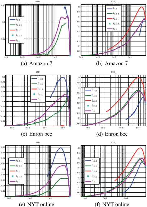
For each of the models we computed class and feature sparsity statistics, specifically the standard deviation of each group sparsity. First, we compute the class sparsity by computing the non zero rates of class terms per feature t: 1c ∑cs=1 I [ωt,c ̸= 0] and then taking the standard deviation of these quantities, denoted by STDc. Second, similarly, we compute the feature sparsity by computing the non zero rates of feature terms per class s: 1d ∑dt=1 I [ωt,c ̸= 0], and then taking the standard deviation of these quantities, denoted by STDf . A low value of STDc indicates that for all features the amount of class sparsity is close to uniform. That is, the number of non-zero elements per row is close to a constant. Similarly, a low STDf indicates a consistent feature sparsity.
Results for three datasets are given in Fig 2. The left panels show STDf vs total amount of non zero rates for three datasets, and the right panels show the STDc vs total amount of non zero rates for the same datasets. In all plots the STD goes to zero when the non zero rates go to zero (high spar- F1 (%)
Precision (%)
71.4
71.2
71
70.8
70.6
70.4
70.2
70
Macro F1 vs. Sparsity
10
20
30
40
50
60
70
80
90
80.8
80.6
80.4
80.2
80
79.8
79.6
79.4
79.2
Sparsity (%)
(a) Macro F1 vs. Sparsity(%)
Macro precision vs. Macro recall
ℓ1,2;1
ℓ1,2;2
ℓ2,1;1
ℓ2,1;2
ℓ1,1
ℓ2,2
68.4 68.6 68.8
69
69.2 69.4 69.6 69.8
70
Recall (%)
(b) Macro Precision vs. Macro Recall
Figure 1: Summary of performance results on 14 multi class tasks
sity), as more and more entries of the model are set to zero.
Focusing on the left panels we see that STDf is zero for ℓ2,1;1 , as this regularization either does not enforce a sparsity of a feature, or cancels the entire feature altogether, and thus there is a constant feature sparsity for all classes. The second best (or uniform) regularization is ℓ1,2;2, then ℓ1,1, and ℓ1,2;1 has the least consistent feature sparsity, as it enforces large amount of zero entries per feature, yet the number of classes is no more than 50 (the options for terms removal are limited).
Moving to the right panels we observe that ℓ1,2;1 has the lowest STDc, then, ℓ1,1 and ℓ1,2;2 are close to each other, and ℓ2,1;1 is with the highest STDc. In both measures, ℓ1,1 STD values are mediocre compared to other regularizations' values which fits its lack of specific sparsity structure. As expected, ℓ1,2;1 has a consistent class sparsity (low STDc) and ℓ1,2;2 has a consistent feature sparsity (low STDf ). However, ℓ1,2;1 has a low feature consistency (high STDf ) while ℓ1,2;2 has a medium class consistency (very close to ℓ1,1). This can be explained, as before, by the fact that c ≪ d, which enables scattered non zero terms for each of the classes, allowing a higher chance for features with a consistent class sparsity. ℓ2,1;2 yields only dense results, hence not relevant for this analysis.
Similar behavior was evident in all other datasets.
6 Conclusions and FutureWork
This work presents a novel approach for multi class problems, proposing an individual feature selection, which is formulated by the ℓ1,2;2 norm regularization. This approach was thoroughly investigated and compared with the common ℓ2,2, ℓ1,1 and ℓ2,1 regularizations, examining performance and sparsity pattern results. The empirical study, conducted on 14 multi class datasets, demonstrates the superiority of the ℓ1,2;2 regularization for the multi class problems, outperforming other regularizations. Interestingly, results for ℓ1,2;2 are not only better, but also sparser than all other regularizations, including the general sparsity promoting ℓ1,1. It was also shown that sparsity patterns fitted the expectations with consistent feature sparsity results for ℓ1,2;2. In addition, theoretical guarantees were proved using robustness and Rademacher analysis. These guarantees supply theoretical reasoning for choosing ℓ1,2;2 norm, given a specific prior knowledge.
Future work may analyze and find criteria for performance advantage of the proposed regularization and further investigate specific loss functions and types of datasets, as well as additional types of problems, e.g. multi task. Another possible direction is exploring combinations (sums) of different regularizations to obtain a mixed effect.
@inproceedings{ijcai2013p256,
  title     = {Multi Class Learning with Individual Sparsity},
  author    = {Vatashsky, Ben Zion and Crammer, Koby},
  booktitle = {Proceedings of the Twenty-Third International Joint Conference on
               Artificial Intelligence, {IJCAI-13}},
  publisher = {AAAI Press / International Joint Conferences on Artificial Intelligence},
  editor    = {Francesca Rossi},
  pages     = {1729--1734},
  year      = {2013},
  month     = {8},
  url       = {https://ijcai.org/proceedings/2013/256},
}
TY - CPAPER TI - Multi Class Learning with Individual Sparsity AU - Vatashsky, Ben Zion AU - Crammer, Koby T2 - Proceedings of the Twenty-Third International Joint Conference on Artificial Intelligence, IJCAI-13 PB - AAAI Press / International Joint Conferences on Artificial Intelligence PY - 2013 SP - 1729 EP - 1734 UR - https://ijcai.org/proceedings/2013/256 ER -Copied
Machine-readable versions of this paper, for tools and AI agents:





