Measuring Statistical Dependence via the Mutual Information Dimension

1 Introduction

How to measure dependence of variables is a classical yet fundamental problem in statistics. Starting with the Galton's work of Pearson's correlation coefficient [Stigler, 1989] for measuring linear dependence, many techniques have been proposed, which are of fundamental importance in scientific fields such as physics, chemistry, biology, and economics.

Machine learning and statistics has defined a number of techniques over the last decade which are designed to measure not only linear but also nonlinear dependences [Hastie et al., 2009]. Examples include kernel-based [Bach and Jordan, 2003; Gretton et al., 2005], mutual informationbased [Kraskov et al., 2004; Steuer et al., 2002], and distancebased [Sz´ekely et al., 2007; Sz´ekely and Rizzo, 2009] methods. Their main limitation in practice, however, is the lack of scalability or that one has to specify the type of nonlinear relationship one is interested in beforehand, which requires non-trivial parameter selection.

Recently, in Science, a distinct method called maximal information coefficient (MIC) has been proposed by Reshef et al. [2011] (further analyzed in [Reshef et al., 2013]) that measures any kind of relationships between two continuous variables. They use the mutual information obtained by discretizing data and, intuitively, MIC is the maximum mutual information across a set of discretization levels.

However, it has some significant drawbacks: First, MIC depends on the input parameter B(n), which is a natural number specifying the maximum size of a grid used for discretization of data to obtain the entropy [Reshef et al., 2011, SOM 2.2.1]. This means that MIC becomes too small if we choose small B(n) and too large if we choose large B(n). Second, it has high computational cost, as it is exponential with respect to the number of data points 1 , and not suitable for large datasets. Third, as pointed out by Simon and Tibshirani [2012], it does not work well for relationship discovery in the presence of noise.

Here we propose to measure dependence between two random variables by the mutual information dimension, or MID, to overcome the above drawbacks of MIC and other machine learning based techniques. First, it contains no parameter in theory and the estimation method proposed in this paper is also parameter-free. Second, its estimation is fast; the average-case time complexity is O(n logn), where n is the number of data points. Third, MID is experimentally shown to be more robust to uniformly distributed noise data than MIC and other methods.

The definition of MID is simple:

for two random variables X and Y , where dimX and dimY are the information dimension of random variables X and Y , respectively, and dimXY is that of the joint distribution of X and Y . The information dimension is one of the fractal dimensions [Ott, 2002] introduced by R´enyi [1959; 1970], and its links to information theory were recently studied [Wu and Verd´u, 2010; 2011]. Although MID itself is not a new concept, this is the first study that introduces MID as a measure of statistical dependence between random variables;

1 Since computing the exact MIC is usually infeasible, they used heuristic dynamic programming for efficient approximation.

to date, MID has only been used for chaotic time series analysis [Buzug et al., 1994; Prichard and Theiler, 1995].

MID has desirable properties as a measure of dependence: For every pair of random variables X and Y , (1) MID(X; Y ) = MID(Y ;X) and 0 ≤ MID(X; Y ) ≤ 1; (2) MID(X; Y ) = 0 if and only if X and Y are statistically independent (Theorem 1); and (3) MID is invariant with respect to translation and scaling (Theorem 3). Furthermore, MID is related to MIC and can be viewed as an extension of it (see Section 2.4).

To estimate MID from a dataset, we construct an efficient parameter-free method. Although the general strategy is the same as the standard method used for estimation of the Boxcounting dimension [Falconer, 2003], we aim to remove all parameters from the method using the sliding window strategy, where the width of a window is adaptively determined from the number of data points. The average-case and the worst-case complexities of our method are O(n logn) and O(n2 ) with the number n of data points, respectively, which is much faster than the estimation algorithm of MIC and the other state-of-the-art methods such as the Hilbert-Schmidt independence criterion (HSIC) [Gretton et al., 2005] and the distance correlation [Sz´ekely et al., 2007] whose time complexities are O(n2 ). Hence MID scales up to massive datasets with millions of data points.

This paper is organized as follows: Section 2 introduces MID and analyzes it theoretically. Section 3 describes a practical estimation method of MID. The experimental results are presented in Section 4, followed by conclusion in Section 5.

2 Mutual Information Dimension

In fractal and chaos theory, dimension has a crucial role since it represents the complexity of an object based on a "measurement" of it. We employ the information dimension in this paper, which belongs to a larger family of fractal dimensions [Falconer, 2003; Ott, 2002].

In the following, let N be the set of natural numbers including 0, Z the set of of integers, and R the set of real numbers. The base of the logarithm is 2 throughout this paper.

We divide the real line R into intervals of the same width to obtain the entropy of a discretized variable. Formally,

for an integer z ∈ Z. We call the resulting system Gk = {Gk(z) | z ∈ Z} the partition of R at level k. Partition for the two-dimensional space is constructed from Gk as G2 k = {Gk(z1) ×Gk(z2) | z1, z2 ∈ Z}.

2.1 Information Dimension

Given a real-valued random variable X, we construct for each level k the discrete random variable Xk over Z, whose probability is given by Pr(Xk = z) = Pr(X ∈ Gk(z)) for each z ∈ Z. We denote the probability mass function for Xk by pk(x) = Pr(Xk = x), and that of the joint probability by pk(x, y) = Pr(Xk = x and Yk = y).

We introduce the information dimension, which intuitively shows the complexity of a random variable X as the ratio comparing the change of the entropy to the change in scale.

Definition 1 (Information Dimension [R´enyi, 1959]) The information dimension of X is defined as

where H(Xk) denotes the entropy of Xk, defined by H(Xk) = - ∑x∈Z pk(x) log pk(x).

The information dimension for a pair of two real-valued variables X and Y is naturally defined as dimXY := limk→∞ H(Xk, Yk)/k, where H(Xk, Yk) = - ∑x∈Z ∑y∈Z pk(x, y) log pk(x, y), the joint entropy of Xk and Yk. Informally, the information dimension indicates how much a variable fills the space, and this property enables us to measure the statistical dependence. Notice that

In this paper, we always assume that dimX and dimY exist and X and Y are Borel-measurable. Our formulation applies to pairs of continuous random variables X and Y . 2

2.2 Mutual Information Dimension

Based on the information dimension, the mutual information dimension is defined in an analogous fashion to the mutual information.

Definition 2 (Mutual Information Dimension) For a pair of random variables X and Y , the mutual information dimension, or MID, is defined as

We can easily check that MID is also defined as

with the mutual information I(Xk; Yk) of Xk and Yk defined as I(Xk; Yk) = ∑x,y∈Z pk(x, y) log(pk(x, y)/pk(x)pk(y)).

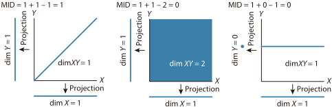
Informally, the larger MID(X; Y ), the stronger the statistical dependence between X and Y . Figure 1 shows intuitive examples of the information dimension and MID.

2 Furthermore, it applies to variables with no singular component in terms of the Lebesgue decomposition theorem [R´enyi, 1959]. In contrast, Reshef et al. [2011] (SOM 6) theoretically analyzed only continuous variables.

2.3 Properties of MID

It is obvious that MID is symmetric MID(X; Y ) = MID(Y ;X) and that 0 ≤ MID(X; Y ) ≤ 1 holds for any pair of random variables X and Y , as the mutual information I(Xk; Yk) in equation (1) is always between 0 and k.

The following is the main theorem in this paper.

Theorem 1 MID(X; Y ) = 0 if and only if X and Y are statistically independent.

Proof. (⇐) Assume that X and Y are statistically independent. From equation (1), it directly follows that MID(X; Y ) = 0 since I(Xk; Yk) = 0 for all k.

(⇒) Assume that X and Y are not statistically independent. We have MID(X; Y ) = dimX - dimX|Y , where dimX|Y = limk→∞H(Xk|Yk)/k with the conditional entropy H(Yk|Xk) = ∑x,y∈Z pk(x, y) log(pk(x)/pk(x, y)). Thus all we have to do is to prove dimX ̸= dimX|Y to show that MID(X; Y ) ̸= 0 holds. From the definition of entropy, dimX = limk→∞-E log p(Xk)/k and dimX|Y = limk→∞-E log p(Xk|Yk)/k, where E denotes the expectation. Since p(Xk) and p(Xk|Yk) go to p(X) and p(X|Y ) when k → ∞, -E log p(Xk) > -E log p(Xk|Yk) if k is large enough. Thus dimX ̸= dimX|Y holds. □

Note that I(Xk; Yk) does not converge to I(X; Y ) (and actually goes to infinity) when X and Y are not statistically independent. It is analogue to the entropy H(Xk) → ∞ as k → ∞ and is different from the differential entropy of X.

We can also characterize functional relationships with an MID score of one.

Theorem 2 Let X be a random variable with an absolutely continuous distribution. For any function f such that f(X) also has an absolutely continuous distribution, MID(X; f (X)) = 1.

Proof. From Theorem 1 in [R´enyi, 1959], it follows that dimX = dimf(X) = 1. Moreover, since H(Xk) = H(Xk, f(Xk)), we have dimXf(X) = dimX = 1. □

Corollary 1 Let X be a random variable with an absolutely continuous distribution. Given finitely many functions f1, f2, . . . , fm such that each fi(X) has an absolutely continuous distribution. For the multivalued function F with F(X) = fi(X) (i ∈ {1, 2, . . . , m}), MID(X; F(X)) = 1.

Ott et al. [1984] provide a detailed analysis of the invariance properties of the information dimension. The translation (shift) and scale invariance of MID directly follow.

Theorem 3 For any a, b ∈ R,

2.4 Comparison toMIC

Here we show the relationship between MID and the maximal information coefficient (MIC) [Reshef et al., 2011]. Let D be a dataset sampled from a distribution (X, Y ), where X and Y are continuous random variables. The dataset D is discretized by a grid G with x rows and y columns, that is, the x-values and the y-values of D are divided into x and y bins, respectively. The probability distribution D|G is induced by D on the grid G, where the probability mass of each cell is the fraction of data points falling into the cell.

The characteristic matrix M(D) is defined as M(D)x,y = I ∗ (D, x, y)/ logmin{x, y}, where I ∗ (D, x, y) is the maximum of the mutual information I(D|G) over all grids G of x columns and y rows. Then, MIC is defined as MIC(D) = maxxy<B(n)M(D)x, y. Here, when n goes to infinity, we can easily check that MID(X; Y ) = limn, x, y→∞M(D)x, y almost surely since D|G → (X, Y ) as n, x, y → ∞ almost surely. Thus we can say that MIC is the maximum value under the constraint xy < B(n) specified by the user, while MID is the limit of M(D) when x, y → ∞.

This difference provides more power of detection to MID, especially for multivalued functions which are referred to as non-functional in [Reshef et al., 2011]. MID is one for such relationships (Corollary 1) as MID focuses on the ratio of the changes in the limit, while MIC does not.

3 Estimation of MID

We construct an estimation method for the information dimension and MID on finite samples. While the information dimension itself has been studied from a theoretical perspective [Ott, 2002; Ott et al., 1984; Wu and Verd´u, 2010], actual estimation of its value from a finite dataset remains a challenge. For this reason, we design a novel estimation method for the information dimension and MID.

In the following, we always assume that data are in the unit interval I = [0, 1] × [0, 1], which can be achieved by normalization. Since MID is translation and scaling invariant, this transformation has no effect on MID.

3.1 Preliminaries

We modify the definition of Gk(z) as follows: the domain dom(Gk) = {0, 1, . . . , 2k - 1}, Gk(z) := [z, z + 1) · 2-k if z ∈ {0, 1, . . . , 2k - 2}, and Gk(z) := [z, z + 1] · 2-k if z = 2k -1. Moreover, we define G2k (z1, z2) := Gk(z1)×Gk(z2) for a pair of integers z1, z2. We write Gk = {Gk(z) | z ∈ dom(Gk) } and G2 k = {G2k (z1, z2) | z1, z2 ∈ dom(Gk) }.

Given a dataset D = {(x1, y1), (x2, y2), . . . , (xn, yn)} sampled from a distribution (X, Y ). We use the natural es- Algorithm 1 Estimation of MID

Input: Dataset D

Output: Estimator of MID

for each Z ∈ {X, Y, (X, Y )} do

Compute H( ˆ Z1), H( ˆ Z2), . . . until each point is isolated; Find the best fitted regression line for k v.s. H( ˆ Zk) for each window of width w (equation (2)) started from s ∈ SZ(w); d(Z) ← the gradient of the obtained line;

end for

Output d(X) + d(Y ) - d(X, Y );

timator ˆXk of Xk, where the probability is defined as

(#A denotes the number of elements of the set A) for all z ∈ dom(Gk), and similarly defined for Pr( ˆ Yk = z) and the joint probability Pr( ˆXk = z1, ˆ Yk = z2). This is the fraction of points in D falling into each cell. Trivially, ˆXk (resp. ˆ Yk) converges to Xk (resp. Yk) almost surely when n →∞.

3.2 Estimation via SlidingWindows

Informally, the information dimension dimX (resp. dimY , dimXY ) can be estimated as the gradient of the regression line over k v.s. the entropy H( ˆXk) (resp. H( ˆ Yk), H( ˆXk, ˆ Yk)) since H( ˆXk) ≃ dimX · k + c such that the difference of the two sides goes to zero as k →∞. This approach is the same as the standard one for the box-counting dimension [Falconer, 2003, Chapter 3]. However, since n is finite, only a finite range of k should be considered to obtain the regression line. In particular, H( ˆXk) is monotonically nondecreasing as k increases and finally it converges to some constant value, where each cell contains at most one data point.

To effectively determine the range of k, we use the sliding window strategy to find the best fitted regression line. We set the width w of each window to the maximum value satisfying

for estimation of dimX or dimY and dimXY , respectively. If |Gw| = 2w > n holds, then there exists a dataset D such that H( ˆXw) -H( ˆXw-1) = 0, and hence we should not take the point (w,H( ˆXw)) into account in the regression for estimating dimX. Hence w in equation (2) gives the upper bound of the width of each window that can be effectively applied to any dataset in estimation of the dimension.

3.3 MID Estimator

Here we give an estimator of MID using the sliding window strategy. For simplicity, we use the symbol Z to represent the random variables X, Y , or the pair (X, Y ).

Let w be the maximum satisfying equation (2) and define

This is the set of starting points of the windows. Note that this set is always finite since H( ˆ Zk) converges. We denote the resulting coefficient by β(s) and the coefficient of determination by R2 (s) when we apply linear regression to the set of w points { (s,H( ˆ Zs)), (s + 1, H( ˆ Zs+1)), . . . , (s + w - 1, H( ˆ Zs+w-1)) }.

Definition 3 (Estimator of information dimension) Given a dataset D. Define the estimator d(Z) (Z = X, Y , or the pair (X, Y )) of the information dimension dimZ as

and define the estimator of MID as

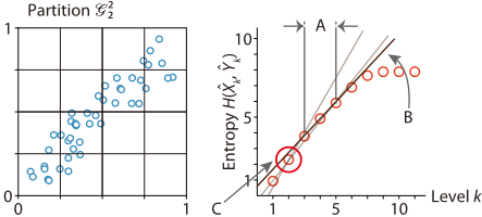
The estimator of MID is obtained by Algorithm 1 and Figure 2 shows an example of estimation. The average-case and the worst-case time complexities are O(n log n) and O(n2 ), respectively, since computation of H( ˆ Zk) takes O(n) for each k and it should be repeated O(logn) and O(n) times in the average and the worst case.

4 Experiments

We evaluate MID experimentally to check its efficiency and effectiveness in detecting various types of relationships, and compare it to other methods including MIC. We use both synthetic data and gene expression data. Moreover, we apply MID to feature selection in nonlinear regression for real data to demonstrate its potential in machine learning applications.

Environment: We used Mac OS X version 10.7.4 with 2 × 3 GHz Quad-Core Intel Xeon CPU and 16 GB of memory. MID was implemented in C 3 and compiled with gcc 4.2.1. All experiments were performed in the R environment, version 2.15.1 [R Core Team, 2012].

Comparison partners: We used Pearson's correlation coefficient (PC), the distance correlation (DC) [Sz´ekely et al., 2007], mutual information (MI) [Kraskov et al., 2004], the Hilbert-Schmidt independence criterion (HSIC) [Gretton et al., 2005], and MIC (heuristic approximation) [Reshef et al., 2011]. DC was calculated by the R energy package; MI and MIC by the official source code 4 ; HSIC was implemented in R (computationally expensive processes were done by efficient packages written in C or Fortran). All parameters in MIC were set to the default values. Gaussian kernels with the width set to the median of the pairwise distances between the samples were used in HSIC, which is a popular heuristics [Gretton et al., 2005; 2008].

3 The source code for MID is available at http://webdav. tuebingen.mpg.de/u/karsten/Forschung/MID

4 MIC: http://www.exploredata.net, MI: http://www.klab.caltech. edu/∼kraskov/MILCA

4.1 Scalability

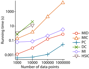
We checked the scalability of each method. We used the linear relationship without any noise, and varied the number n of data points from 1, 000 to 1, 000, 000.

Results of running time are shown in Figure 3 (we could not calculate DC and HSIC for more than n = 100, 000 due to their high space complexity O(n2 )). These results clearly show that on large datasets, MID is much faster than other methods including MIC which can detect nonlinear dependence. Notice that time complexities of MIC, DC, and HSIC are O(n2 ). PC is faster than MID, but unlike MID, it cannot detect nonlinear dependence.

4.2 Effectivity inMeasuring Dependence

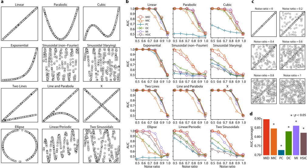
First, we performed ROC curve analysis using synthetic data to check both precision and recall in detection of various relationship types in the presence of uniformly distributed noise data. We prepared twelve types of relationships shown in Figure 4a, same datasets were used in [Reshef et al., 2011]. For generation of noisy datasets, we fixed the ratio of uniformly distributed noise in a dataset in each experiment, and varied from 0 to 1. Figure 4c shows examples of linear relationships with noise (n = 300). For instance, if the noise ratio is 0.5, 150 points come from the linear relationship, and the remaining 150 points are uniformly distributed noise.

We set the number of data points n = 300. In each experiment, we generated 1000 datasets, where 500 are sampled from the relationship type with noise (positive datasets), and the remaining 500 sets are just noise, that is, composed of statistically independent variables (negative datasets). Then, we computed the AUC score from the ranking of such 1000 datasets. Thus both precision and recall are taken into account, while Reshef et al. [2011] evaluated only recall.

Figure 4b shows results of ROC curve analysis for each relationship type. We omit results for noise ratio from 0 to 0.4 since all methods except for PC have the maximum AUC in most cases. In more than half of the cases, MID showed the best performance. Specifically, the performance of MID was superior to MIC in all cases except for two sinusoidal types. Moreover, although MI showed better performance than MID in four cases, its performance was much worse than MID and MIC in sinusoidal types. In addition, MI is not normalized, hence it is difficult to illustrate the strength of dependence in the real world situations, as mentioned by Reshef et al. [2011]. In contrast to MI, MID showed reasonable performance in all relationship types. Since MID was shown to be much faster than MIC, DC, and MI, these results indicate that MID is the most appropriate among these methods for measuring dependence in massive data. Note that MIC's performance is often worst except for sinusoidal types, which confirms the report by Simon and Tibshirani [2012].

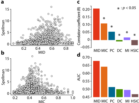
Figure 4d is the average of the means of AUC over all relationship types (noise ratio from 0.5 to 0.9 were taken into account). The score of MID was significantly higher than other methods (the Wilcoxon signed-rank test, α = 0.05).

Next, we evaluated MID using the cdc15 yeast (Saccharomyces cerevisiae) gene expression dataset from [Spellman et al., 1998], which was used in [Reshef et al., 2011] and contains 4381 genes 5 . This dataset was originally analyzed to identify genes whose expression levels oscillate during the cell cycle. We evaluated dependence between each time series against time in the same way as [Reshef et al., 2011, SOM 4.7]. The number n = 23 for each gene.

Figure 5a, b illustrate scatter plots of MID and MIC versus Spellman's score. We observe that genes with high Spellman's scores tend to have high MID scores: the correlation coefficient (R) between Spellman's scores and MID was significantly higher than others (α = 0.05, Figure 5c).

To check both precision and recall in real data, we again performed ROC curve analysis. That is, we first ranked genes by measuring dependence, followed by computing the AUC score. Genes whose Spellman's scores are more than 1.314 were treated as positives as suggested by Spellman et al. [1998]. Figure 5d shows the resulting AUC scores. It confirms that MID is the most effective compared to other methods in measuring dependence. The AUC score of PC is low since it cannot detect nonlinear dependence. DC, MI, and HSIC also show low AUC scores. The reason might be the lack of power for detection due to the small n.

4.3 Effectivity in Feature Selection

Finally, we examined MID as a scoring method for feature selection. To illustrate the quality of feature selection, we performed kNN regression using the selected features to estimate the nonlinear target function, where the average of the k nearest neighbors is calculated as an estimator for each data point (k was set to 3). We measured the quality of prediction by the mean squared error (MSE). For each dataset, we generated training and test sets by 10-fold cross validation and performed feature selection using only the training set. Eight real datasets were collected from UCI repository [Frank and Asuncion, 2010] and StatLib 6 .

5 http://www.exploredata.net/Downloads/Gene-ExpressionData-Set

We adopted the standard filter method, that is, we measured dependence between each feature and the target variable, and produced the ranking of the features from the training set. We then applied kNN regression (based on the training set) to the test set repeatedly, varying the number of selected top ranked features. Results for each dataset are shown in Figure 6a, and the average R2 , which is the correlation between predicted and target values over all datasets, is summarized in Figure 6b. MID performed significantly better than any other methods (the Wilcoxon signed-rank test, α = 0.05).

5 Conclusion

We have developed a new method based on dimension theory for measuring dependence between real-valued random variables in large datasets, the mutual information dimension (MID). MID has desirable properties as a measure of dependence, that is, it is always between zero and one, it is zero if and only if variables are statistically independent, and it is translation and scaling invariant. Moreover, we have constructed an efficient parameter-free estimation method for MID, whose average-case time complexity is O(n logn). This method has been experimentally shown to be scalable and effective for various types of relationships, and for nonlinear feature selection in regression.

6 http://lib.stat.cmu.edu/datasets/

MID overcomes the drawbacks of MIC: (1) MID contains no parameter; (2) MID is fast and scales up to massive datasets; and (3) MID shows superior performance in detecting relationships in the presence of uniformly distributed noise. In [Reshef et al., 2011], an additive noise model was considered; MID might not work well for this type of noise model. Since MID is based on dimension theory, it tends to judge that the true distribution is a two-dimensional plane, with no dependence. We will further explore the exciting connection between dimension theory and statistical dependence estimation to address this challenge.