
Multiple Task Learning Using Iteratively Reweighted Least Square
Proceedings of the Twenty-Third International Joint Conference on Artificial Intelligence. Pages 1607-1612.
© 2013 International Joint Conferences on Artificial Intelligence
Abstract
Multiple task learning (MTL) is becoming popular due to its theoretical advances and empirical successes. The key idea of MTL is to explore the hidden relationships among multiple tasks to enhance learning performance. Recently, many MTL algorithms have been developed and applied to various problems such as feature selection and kernel learning. However, most existing methods highly relied on certain assumptions of the task relationships. For instance, several works assumed that there is a major task group and several outlier tasks, and used a decomposition approach to identify the group structure and outlier tasks simultaneously. In this paper, we adopt a more general formulation for MTL without making specific structure assumptions. Instead of performing model decomposition, we directly impose an elastic-net regularization with a mixture of the structure and outlier penalties and formulate the objective as an unconstrained convex problem. To derive the optimal solution efficiently, we propose to use an Iteratively Reweighted Least Square (IRLS) method with a preconditioned conjugate gradient, which is computationally affordable for high dimensional data. Extensive experiments are conducted over both synthetic and real data, and comparisons with several state-of-the-art algorithms clearly show the superior performance of the proposed method.
- [Ando and Zhang, 2005] Rie Kubota Ando and Tong Zhang. A framework for learning predictive structures from multiple tasks and unlabeled data. JMLR, 6:1817-1853, 2005.
- [Argyriou et al., 2008] Andreas Argyriou, Theodoros Evgeniou, and Massimiliano Pontil. Convex multi-task feature learning. MACH LEARN, 73(3):243-272, 2008.
- [Bakker and Heskes, 2003] Bart Bakker and Tom Heskes. Task clustering and gating for bayesian multitask learning. JMLR, 4:83-99, 2003.
- [Bickel et al., 2008] Steffen Bickel, Jasmina Bogojeska, Thomas Lengauer, and Tobias Scheffer. Multi-task learning for hiv ther- apy screening. In ICML, 2008.
- [Caruana, 1997] Rich Caruana. Multitask learning. MACH LEARN, 28(1):41-75, 1997.
- [Chen et al., 2009] Jianhui Chen, Lei Tang, Jun Liu, and Jieping Ye. A convex formulation for learning shared structures from multiple tasks. In ICML, 2009.
- [Chen et al., 2011] Jianhui Chen, Jiayu Zhou, and Jieping Ye. In- tegrating low-rank and group-sparse structures for robust multi- task learning. In SIGKDD, 2011.
- [Daubechies et al., 2008] Ingrid Daubechies, Ronald Devore, Mas- simo Fornasier, and C. Sinan Gntrk. Iteratively reweighted least squares minimization for sparse recovery. Comm. Pure Appl. Math, 2008.
- [Ghosn and Bengio, 1996] Joumana Ghosn and Yoshua Bengio. Multi-task learning for stock selection. In NIPS, 1996.
- [Gong et al., 2012] Pinghua Gong, Jieping Ye, and Changshui Zhang. Robust multi-task feature learning. In SIGKDD, 2012.
- [Jacob et al., 2008] Laurent Jacob, Francis Bach, and Jean-Philippe Vert. Clustered multi-task learning: A convex formulation. In NIPS, 2008.
- [Jalali et al., 2010] Ali Jalali, Pradeep D. Ravikumar, Sujay Sang- havi, and Chao Ruan. A dirty model for multi-task learning. In NIPS, 2010.
- [Kang et al., 2011] Zhuoliang Kang, Kristen Grauman, and Fei Sha. Learning with whom to share in multi-task feature learn- ing. In ICML, 2011.
- [Kim and Xing, 2010] Seyoung Kim and Eric P. Xing. Tree-guided group lasso for multi-task regression with structured sparsity. In ICML, 2010.
- [Lawrence and Platt, 2004] Neil D. Lawrence and John C. Platt. Learning to learn with the informative vector machine. In ICML, 2004.
- [Liu et al., 2009] Jun Liu, Shuiwang Ji, and Jieping Ye. Multi-task feature learning via efficient ℓ2,1-norm minimization. In UAI, 2009.
- [Lounici et al., 2009] Karim Lounici, Massimiliano Pontil, Alexan- dre B. Tsybakov, and Sara A. van de Geer. Taking advantage of sparsity in multi-task learning. In COLT, 2009.
- [Negahban and Wainwright, 2008] Sahand Negahban and Martin J. Wainwright. Joint support recovery under high-dimensional scal- ing: Benefits and perils of ℓ1,∞-regularization. In NIPS, 2008.
- [Negahban and Wainwright, 2010] Sahand Negahban and Martin J. Wainwright. Estimation of (near) low-rank matrices with noise and high-dimensional scaling. In ICML, 2010.
- [Parameswaran and Weinberger, 2010] S. Parameswaran and K.Q. Weinberger. Large margin multi-task metric learning. In NIPS, 2010.
- [Pong et al., 2010] Ting Kei Pong, Paul Tseng, Shuiwang Ji, and Jieping Ye. Trace norm regularization: Reformulations, algo- rithms, and multi-task learning. SIAM J. Optim., 20(6):3465- 3489, 2010.
- [Rao and Kreutz-Delgado, 1999] Bhaskar D. Rao and Kenneth Kreutz-Delgado. An affine scaling methodology for best basis selection. IEEE Trans. Image Process, 47(1):187-200, 1999.
- [Rao et al., 2003] Bhaskar D. Rao, Kjersti Engan, Shane F. Cotter, Jason Palmer, and Kenneth Kreutz-delgado. Subset selection in noise based on diversity measure minimization. IEEE Trans. Sig- nal Process, pages 760-770, 2003.
- [Saad, 2003] Y. Saad. Iterative Methods for Sparse Linear Sys- tems. Society for Industrial and Applied Mathematics, 2nd edi- tion, 2003.
- [Schwaighofer et al., 2004] Anton Schwaighofer, Volker Tresp, and Kai Yu. Learning gaussian process kernels via hierarchical bayes. In NIPS, 2004.
- [Thrun and Sullivan, 1996] Sebastian Thrun and Joseph O Sullivan. Discovering structure in multiple learning tasks: The tc algo- rithm. In ICML, 1996.
- [Wang et al., 2009] Xiaogang Wang, Cha Zhang, and Zhengyou Zhang. Boosted multi-task learning for face verification with ap- plications to web image and video search. In CVPR, 2009.
- [Wang et al., 2011] Hua Wang, Feiping Nie, Heng Huang, Shan- non L. Risacher, Chris H. Q. Ding, Andrew J. Saykin, Li Shen, and Adni. Sparse multi-task regression and feature selection to identify brain imaging predictors for memory performance. In ICCV, 2011.
- [Xue et al., 2007] Ya Xue, Xuejun Liao, Lawrence Carin, and Bal- aji Krishnapuram. Multi-task learning for classification with dirichlet process priors. JMLR, 8:35-63, 2007.
- [Yang et al., 2009] Xiaolin Yang, Seyoung Kim, and Eric P. Xing. Heterogeneous multitask learning with joint sparsity constraints. In NIPS, 2009.
- [Yu et al., 2005] Kai Yu, Volker Tresp, and Anton Schwaighofer. Learning gaussian processes from multiple tasks. In ICML, 2005.
- [Zhang and Yeung, 2010] Yu Zhang and Dit-Yan Yeung. Transfer metric learning by learning task relationships. In SIGKDD, 2010.
- [Zhang et al., 2005] Jian Zhang, Zoubin Ghahramani, and Yiming Yang. Learning multiple related tasks using latent independent component analysis. In NIPS, 2005.
- [Zhang et al., 2010] Yu Zhang, Dit-Yan Yeung, and Qian Xu. Prob- abilistic multi-task feature selection. In NIPS, 2010.
- [Zhou et al., 2011] Jiayu Zhou, Lei Yuan, Jun Liu, and Jieping Ye. A multi-task learning formulation for predicting disease progres- sion. In SIGKDD, 2011.
- [Zou and Hastie, 2003] Hui Zou and Trevor Hastie. Regularization and variable selection via the elastic net. J. R. Stat. Soc. Ser. B Stat. Methodol., 67(2):301-320, 2003.
References were extracted automatically from the PDF and may contain errors.
Full text extracted automatically from the PDF; figures, tables and equations may differ. The PDF is the version of record.
1 Introduction
Multiple task learning (MTL) aims to improve the learning performance through training multiple models jointly and simultaneously. It is particularly useful if there exist intrinsic relationships among multiple learning tasks and the training data is inadequate for each single task. Due to its empirical successes, MTL has been applied to various application domains, including social media categorization and search [Chen et al., 2009; Wang et al., 2009], disease modeling and prediction [Bickel et al., 2008; Zhou et al., 2011], and even financial stock selection [Ghosn and Bengio, 1996].
One fundamental assumption of MTL is model commonality between the multiple learning tasks. Typically, such commonality can be represented as shared common structures or parameters by the learned models. For instance, structure commonality includes low rank subspace sharing [Negahban and Wainwright, 2010; Pong et al., 2010] and feature set sharing [Argyriou et al., 2008; Kim and Xing, 2010; Liu et al., 2009; Lounici et al., 2009; Negahban and Wainwright, 2008; Yang et al., 2009; Zhang et al., 2010]. In terms of the parameter commonality, it includes a wide range of options depending on the used learning methods, such as the hidden units in neural networks [Caruana, 1997], the priors in hierarchical Bayesian models [Bakker and Heskes, 2003; Schwaighofer et al., 2004; Yu et al., 2005; Zhang et al., 2005], the parameters in Gaussian process covariance [Lawrence and Platt, 2004], the feature mapping matrices [Ando and Zhang, 2005], and the similarity metrics [Parameswaran and Weinberger, 2010; Zhang and Yeung, 2010]. Through exploring these model commonalities, either structures or parameters, simultaneously learning multiple tasks will benefit from the learning of each other. Hence, the MTL paradigm often achieves better generalization performance than independently learning a prediction model for each task.
However, the model commonality is a fairly strong assumption, which is often invalid in real applications. Therefore, two compromised yet more realistic scenarios, i.e., task grouping and task outlier, have been explored recently. For task grouping, one assumes that the commonality only exists among tasks within the same group. During the learning process, through identifying such task groups, the unrelated tasks from different groups will not influence each other [Jacob et al., 2008; Kang et al., 2011; Thrun and Sullivan, 1996; Xue et al., 2007]. In the task outlier scenario [Chen et al., 2011], a robust MTL algorithm was proposed to capture the commonality for a major group of tasks while detecting the outlier tasks. A popular way to tackle the robust MTL problem is to use a decomposition framework, which forms the learning objective with a structure term and an outlier penalty term. To efficiently solve the optimization problem, the target model can be further decomposed into two components, reflecting the major group structure and the outliers [Jalali et al., 2010]. Representative decompositions for the major task group include the low-rank structure [Chen et al., 2011] and the group sparsity [Gong et al., 2012].
Note that the aforementioned assumptions of task grouping and task outlier were exclusively considered in most of the existing works. In other words, the task grouping based methods neglected the existence of outlier tasks and many robust MTL framework only assumed the case of one major task group peppered with a few outlier tasks. In this paper, we address MTL under a very general setting where multiple major task groups and outlier tasks could occur simultaneously. In particular, without decomposing the target model, we directly impose an elastic-net regularization with a mixture of structure and outlier penalties. The final objective is formulated as an unconstrained convex problem and an efficient Iteratively Reweighted Least Square (IRLS) method is applied to derive the optimal solution. In addition, we provide theoretical analysis on both convergence and performance bound of the proposed MTL method. Finally, empirical studies on both synthetic and real benchmark datasets corroborate that the proposed MTL learning method clearly outperforms several state-of-the-art MTL approaches.
2 Decomposition Framework of Robust MTL
We first define notations and then briefly introduce the decomposition based robust MTL approach. The dataset is represented as a matrix X ∈ Rd×n , where the column vector xi ∈ Rd is the i-th data point and d is the dimension. In addition, we denote xi· as the i-th row of X, which corresponds to the i-th feature of the data. In a typical setting of multiple task regression or classification, we are given L tasks associated with training data {(X1, y1), · · · , (XL, yL)}, where Xl ∈ Rd×nl , yl ∈ Rnl are the input and response of the l-th task with a total of nl samples. The objective of MTL is to derive optimal prediction models for all the tasks simultaneously. In particular, for linear regression models, the prediction model for the l-th task is represented as f(wl,Xl) = X⊤l wl. We then use a coefficient matrixW= [w1,w2, · · · ,wL] to represent all the regression tasks.
As mentioned earlier, the key idea of the decomposition framework is to assume that the target model W can be represented by the supposition of a block-structured component P with row-sparsity and a outlier component Q with elementwise sparsity [Jalali et al., 2010], i.e., W = P +Q. Then the objective for robust MTL can be formed as the following optimization problem with the two types of sparsity regularization:
where pl and ql are the l-th column vectors of P and Q, respectively. The linear prediction model is written as
with a quadratically formed empirical loss
The above decomposition based objective can be efficiently optimized via various techniques, such as an accelerated gradient descent method [Gong et al., 2012]. However, this formulation does not consider the case with multiple groups of tasks, whose structures cannot be simply represented as a single block-structured component. In addition, although the early work provided the error bounds of recovering the two decomposed parts P,Q [Gong et al., 2012], the error bound for recovering the true target model W remains unrevealed.
3 The Proposed Algorithm: MTL-IRLS
Here, we will first describe a general MTL formulation without specific assumptions of the tasks' structure. Then we will propose an efficient solution using the IRLS algorithm.
3.1 Formulation
In this paper, we consider using the linear regression model for learning L tasks simultaneously. As described earlier, the prediction function for the l-th task is represented as f(Xl) = X⊤l wl, l = 1, 2, · · · , L. Motivated by the existing works in the MTL [Jalali et al., 2010; Gong et al., 2012], we formulate a minimization problem with the cost function as a regularized quadratic loss:
where J(W) is a structure penalty term and λ is the coefficient of the regularization term. Without using the supposition assumption to decompose W into two structure terms, here we use a convex mixture of lasso and ridge regularization of the coefficient matrix, which has been introduced as the elastic-net regularization in [Zou and Hastie, 2003]. Specifically, the regularization term reflects a combination of a structure inducing norm and an outlier detecting norm as:
Here γ ∈ [0, 1] is a constant to balance the two norms. Note that for the non-degenerate setting with γ ∈ (0, 1), the mixture of these two structure norms is strictly convex, and the coefficient matrix W exhibits the characteristics of both row sparse structure and outlier detection. Replacing the regularization term in Eq. 1 by the definition in Eq. 2, we can obtain the following regularized convex cost function:
where the constant coefficients are absorbed as λ1 = λ(1-γ) and λ2 = λγ. Instead of decomposing the target model into a fixed combination of structure and outlier components, the above formulation directly leverages the structure penalty into the cost function without imposing any specific assumptions. Such a formulation is shown to be more flexible in terms of handling various types of tasks, including both grouped tasks and outlier tasks. A similar cost function with the elastic-net regularization term has been used to formulate a sparse regression and feature selection process for brain imaging application [Wang et al., 2011]. However, their solution relies on iteratively solving the inverse of a gram matrix, which is computationally infeasible for high dimensional data. In below, we will present an efficient IRLS approach to perform the training process for the general MTL.
3.2 Solution
We now describe the method for minimizing the cost function in Eq. 3. Adopting the factored representation for the gradient vector of the regularizer [Rao and Kreutz-Delgado, 1999], we can zero the partial derivatives ∂L ∂wl to derive the optimal solution:
where Πl is a diagonal matrix with the element (Πl)ii defined as:
Apparently, the element (Πl)ii consists of two components. The first component ‖wi·‖-1 2 represents the group impact since it imposes row sparsity on the i-th row of W. The second component |wil|-1 represents the individual impact by measuring the impact of the i-th feature on the l-th task. The parameter γ balances the impacts of these two components to the diagonal matrix Π. After performing some manipulations, we can obtain the following equation:
The above equation actually indicates a solution for the following weighted least square problem [Daubechies et al., 2008].
To solve the linear system in Eq. 4, it requires to compute the inverse of a d × d matrix, where a standard algorithm has a complexity of O(n3 ). To derive a feasible solution for high dimension data, we first reformulate Eq. 4 as a preconditioned linear system using Jacobi method [Saad, 2003]:
whereMl = diag(XlX⊤l + λ2 Πl). Although Jacobi iteration can be directly employed to solve Eq. 6, a certain condition on matrix (XlX⊤l + λ2 Πl) is required to receive the convergence guarantee. Here, we use a preconditioned conjugate gradient (PCG) algorithm which provides better asymptotic performance in solving the linear system.
Note that the diagonal matrix Πl can be interpreted as a weight matrix since it essentially enforces different weights to different feature dimensions, i.e., each element of wl. In addition, the calculation of the weight matrix Πl depends on the current wl, which suggests an iterative algorithm to derive the optimal wl. Specifically, in each iteration, we first use the PCG algorithm to solve a preconditioned linear system (equivalent to the weighted least square problem in Eq. 5), and then recalculate the weight matrix Πl. Hence, such an optimization procedure is a typical iteratively reweighted least square method [Daubechies et al., 2008]. Algorithm 1 summarizes the proposed MTL-IRLS method, which is formed in nested loops. The outer loop (while-loop) is for pursuing global convergence and the inner loop (for-loop) is for updating each single task. The weight matrices {Π0l }Ll=1 are initialized as identity matrices, which give equal weights to each dimension for all the tasks.
Algorithm 1 MTL-IRLS
Require: Xl: data matrix of the lth task; yl: response of the lth task;
- 1: Initialize {Π0l }Ll=1 with the identity matrix;
- 2: while not converged do
- 3: for l = 1 to L do
- 4: Update the matrixMl: Ml = diag(XlX⊤l + λ2 Πkl );
- 5: Solve the preconditioned linear system using PCG: M-1 l (XlX⊤l + λ2 Πkl )wl = M-1 l Xlyl;
- 6: Update the weight matrix: Πk+1 l = diag ((1 - γ)‖wi·‖-1 2 +γ|wil|-1 );
- 7: end for
- 8: Update the iteration counter: k = k +1
- 9: end while
3.3 Analysis and Discussion
This subsection provides further analysis to elaborate how the proposed algorithm groups major tasks and identifies outlier tasks simultaneously. To simplify the analysis, we let X ∈ RdL×∑l nl be a block diagonal matrix with Xl ∈ Rd×nl as the l-th block. Define a vectorization operator "vec" over an arbitrary matrix Z ∈ Rd×L as vec(Z) = [z⊤1 , · · · , z⊤l , · · · , z⊤L ]⊤, where zl is the l-th column vector of Z. Then for a single while-loop in Algorithm 1, it can be viewed as solving a weighted least square problem:
where Π ∈ RdL×dL is a concatenated diagonal matrix with Πl as the l-th block. Recall the definition of Πl in Eq. 4, the (ld + i)-th diagonal element of Π is computed as:
which indicates the weight of the i-th feature for the l-th task. We simply assume a balanced case with equal emphasis on row and element-wise sparsity. Note that if both ‖wi·‖ and wil are small, the value Πld+i,ld+i becomes large. Thus, it imposes a heavy penalty for the i-th feature of the l-th task. As a result, the value of wil becomes even smaller after each iteration of the updates. This indeed helps maintain both group sparsity and element-wise sparsity since the i-th feature is not chosen by either the grouped tasks or the outlier tasks. On the other hand, large values of both terms will make Πld+i,ld+i becoming small and impose a slight penalty that encourages the increase of wil after each iteration. It is clear that the iterative algorithm helps recover the group structure which the l-th task belongs to.
The other two complicated cases are that the i-th feature is only relevant to the l-th task while irrelevant to all the other tasks, or the i-th feature is only irrelevant to the l-th task but relevant to all the others. In both cases, the l-th task will be identified as an outlier. If wil is small and ‖wi·‖2 is large, the current task considers this feature as irrelevant while the other tasks consider it as an important feature. Apparently, the penalty Πld+i,ld+i will become large and encourage the updated wil to become smaller. Thus, it further helps identify outlier tasks. If the i-th feature is relevant to the l-th task while irrelevant to the others, the value of wil is large. However, ‖wi·‖2 will not be very small since it also counts the value of wij and satisfies ‖wi·‖2 = (∑Lj=1 w2 ij )1/2 ≥ wil. Hence, the value wil will remain fairly large after each iteration, which means that the element-wise sparsity is still preserved. In summary, the iterative reweighting scheme also provides a unique power for identifying the outlier tasks.
4 Convergence and Performance Bound
We also provide theoretical analysis of the convergence as well as the error bound of the proposed MTL-IRLS algorithm. We start by presenting the lemma in [Rao et al., 2003].
Lemma 1. Given two d-dimentional vectors x = [x1 · · · xd]⊤ and y = [y1 · · · yd]⊤, define E(x) = ∑di=1 |xi| and E(y) = ∑di=1 |yi|, then the following inequation holds
where C = diag{c11, · · · , cii, · · · , cdd} is a diagonal matrix with cii = |xi|-1 .
We will use the above lemma to prove the convergence of the MTL-IRLS algorithm as following. Since it is straightforward to see that the cost function L(W) defined in Eq. 3 is lower bounded as L(W) ≥ 0, we only need to show the monotonic property of the cost function.
Theorem 1. In the proposed MTL-IRLS algorithm, the regularized cost function L(W) decreases monotonically, i.e., L(Wk+1 ) ≤ L(Wk ).
Proof. We have shown that the proposed algorithm minimizes the following weighted least square problem:
Decompose the diagonal matrix Π into two diagonal matrices as: Π = Φ + Ψ (Φ,Ψ ∈ RdL×dL), where the diagonal elements of Φ and Ψ are defined as:
Let us denote a column vector e = [e1, · · · , ed]⊤ with the element ei = ‖wi·‖2 and a diagonal matrix ˆΦ = diag{ˆΦ11, · · · , ˆΦii, · · · , ˆΦdd} with ˆΦii = (1 - γ)‖wi·‖-1 2 . Then we can derive the weighted ℓ2 penalty term of Eq. 7 as:
For simplicity, we denote a dL-dimensional vector v = vec(W). Recalling Eq. 2 and using Lemma 1, we can connect the mixture norm J (W) with the weighted ℓ2 penalty:
Adding the same quadratic empirical loss term to the both sides of the above inequality, then it becomes L(Wk+1 ) - L(Wk ) ≤ G(Wk+1 ) - G(Wk ). Since the IRLS algorithm guarantees G(Wk+1 ) - G(Wk ) < 0, it is easy to see L(Wk+1 ) - L(Wk ) ≤ 0. Hence the convergence of the original cost function is proved.
To further explore the performance bound, we define two index sets for the nonzero and zero rows of matrixW:
Then, we make the following assumption about the training data and the weight matrix, which is a generalized case of the restricted eigenvalue assumption.
Assumption 1. For a matrix Γ ∈ Rd×L, let s ≤ d and t ≤ L. We assume that there exist constants κ1(s) and κ2(t) such that
where the restricted set R(s, t) is defined as:
where |I| counts the number of elements in the set I.
Note that Assumption 1 is similar to the assumptions made by some previous works on MTL [Chen et al., 2011; Gong et al., 2012]. The following theorem gives a bound to measure how well our proposed method can approximate the true W matrix defined in Eq. 3.
Theorem 2. Let ˆW be the optimal solution of Eq. 3 for L ≥ 2 and n, d ≥ 1, and W∗ be the oracle solution. The regularization parameters λ1 and λ2 are chosen as
where b is a positive scalar. Then under Assumption 1, the following results hold with a probability of at least 1 - exp(- 12 (b - dL log(1 + b dL )))
We omit the detailed proof of the above bound due to space limit. However, a similar sketch of the proof can be referred to [Gong et al., 2012], where the authors provided the performance bounds for each decomposed matrix component.
5 Experiments
We conduct experiments on both synthetic and real data to evaluate the effectiveness of our approach. We compare with several state-of-the-art MTL methods, including grouping based MTL (GMTL) [Kang et al., 2011], dirty MTL (DMTL) [Jalali et al., 2010], robust MTL (RMTL) [Chen et al., 2011] and robust multi-task feature learning (rMTFL) [Gong et al., 2012], using the codes from the corresponding authors (except that DMTL codes are from the authors of [Gong et al., 2012]). Performance is measured by both normalized mean squared error (nMSE) and averaged mean squared error (aMSE). We partition the data into training, validation and test sets, and report the mean and standard deviation of the errors of 10 random trials.
5.1 Synthetic Data
We first describe the procedure of synthetic data generation. We set the number of tasks L = 50, and each task has 50 300-dimensional samples. The indices of the nonzero entries for both grouped tasks and outlier tasks are chosen independently from a discrete uniform distribution, and the values of all these nonzero entries are chosen randomly from a standard Gaussian distribution. The data matrices {Xl}Ll=1 are sampled from a standard Gaussian distribution. The response is computed as yl = XTl wl + ξl. Here ξl is a Gaussian noise with zero mean and the variance σ2 l specified by a certain SNR level as σ2 l = 1 nl ‖yl‖2 10-SNR/10 .
| Measure | SNR | GMTL | DMTL | RMTL | rMTFL | MTL-IRLS |
|---|---|---|---|---|---|---|
| nMSE | 20dB | 1.4344 ±0.0642 | 0.6169 ±0.0244 | 0.5806 ±0.0199 | 0.6497 ±0.0243 | 0.5832 ±0.0226 |
| 30dB | 1.4803 ±0.0645 | 0.6007 ±0.0113 | 0.6549 ±0.0274 | 0.5748 ±0.0728 | 0.4315 ±0.0213 | |
| 40dB | 1.1957 ±0.0467 | 0.4588 ±0.0124 | 0.4895 ±0.0137 | 0.4189 ±0.0640 | 0.3242 ±0.0176 | |
| 50dB | 1.2253 ±0.791 | 0.4821 ±0.0236 | 0.5211 ±0.0217 | 0.4147 ±0.0263 | 0.3374 ±0.0219 | |
| aMSE | 20dB | 0.1032 ±0.0046 | 0.0444 ±0.0019 | 0.0418 ±0.0015 | 0.0468 ±0.0019 | 0.0420 ±0.0018 |
| 30dB | 0.0927 ±0.0032 | 0.0376 ±0.0011 | 0.0410 ±0.0019 | 0.0360 ±0.0048 | 0.0270 ±0.0012 | |
| 40dB | 0.0980 ±0.0035 | 0.0376 ±0.0011 | 0.0401 ±0.0014 | 0.0344 ±0.0058 | 0.0266 ±0.0013 | |
| 50dB | 0.0965 ±0.0061 | 0.0380 ±0.0022 | 0.0411 ±0.0022 | 0.0327 ±0.0023 | 0.0266 ±0.0019 |
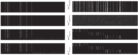
We start from a simple case where the ground truth coefficient matrix contains one major task group and 10 outlier tasks. In particular, the 40 tasks in the major group share no features with the outlier tasks. Figure 1(left) illustrates the recovered coefficient matrices of DMTL, rMTFL and MTLIRLS. It can be seen that all these three methods can recover the nonzero patterns to some extent. Notice that the recovered matrix of the DMTL method contains too many nonzero entries, and rMTFL successfully recovers the entries of the major task group but fails to identify or recover the outlier tasks. In contrast, MTL-IRLS is able to simultaneously recover the major task group and identify the outlier tasks. In addition, we also demonstrate the ability of our approach to handle a more complicated case with three major task groups and five outlier tasks, where each major group contains 15 tasks. As shown in Figure 1(right), the proposed MTL-IRLS is able to recover the coefficient matrix of the major tasks and identify the outlier tasks simultaneously.
Besides the visualized results, we also compute the values of nMSE and aMSE for all the tested cases. In particular, we add in noises with different SNR levels, ranging from 20dB to 50dB, and report the results in Table 1. Apparently, reducing the noise level by increasing the SNR will clearly improve the performance. In most of the cases, the proposed MTL-IRLS provides significantly better performance with lower estimation errors, except that for 20dB it performs similar to RMTL.
5.2 Real Data
The first real dataset used in the experiments is SARCOS, collected from an inverse dynamics prediction problem of a seven degrees-of-freedom anthropomorphic robot arm. The data set consists of 48, 933 observations corresponding to 7 joint torques; each of the observations is described by 21 features including 7 joint positions, 7 joint velocities, and 7 joint accelerations. The goal here is to construct mappings from each observation to the 7 joint torques. Following the setup of existing works, we randomly select 50, 100, 150 observations to form 3 training sets and use 200 and 5, 000 observations as validation and test sets. In addition, we also apply all the methods to the School dataset, which was obtained from the Inner London Education Authority. The data set consists of exam scores of 15, 362 students from 139 secondary schools. Each student is described by 27 attributes such as year, gender and examination score. Following prior works, we vary the ratio of training set as 10%, 20%, 30% respectively, fix the validation ratio as 30%, and use the rest for testing.
| Measure | Training # | GMTL | DMTL | RMTL | rMTFL | MTL-IRLS |
|---|---|---|---|---|---|---|
| nMSE | 50 | 0.0669 ±0.0078 | 0.0668 ±0.0088 | 0.0721 ±0.0081 | 0.0749 ±0.0264 | 0.0565 ±0.0055 |
| 100 | 0.0457 ±0.0020 | 0.0474 ±0.0036 | 0.0575 ±0.0266 | 0.0474 ±0.0024 | 0.0427 ±0.0014 | |
| 150 | 0.0402 ±0.0012 | 0.0426 ±0.0020 | 0.0427 ±0.0013 | 0.0427 ±0.0019 | 0.0390 ±0.0014 | |
| aMSE | 50 | 0.0633 ±0.0074 | 0.0632 ±0.0083 | 0.0683 ±0.0076 | 0.0709 ±0.0250 | 0.0535 ±0.0052 |
| 100 | 0.0433 ±0.0019 | 0.0449 ±0.0034 | 0.0544 ±0.0252 | 0.0449 ±0.0022 | 0.0404 ±0.0013 | |
| 150 | 0.0380 ±0.0012 | 0.0403 ±0.0019 | 0.0404 ±0.0013 | 0.0404 ±0.0018 | 0.0370 ±0.0013 |
| Measure | Training % | GMTL | DMTL | RMTL | rMTFL | MTL-IRLS |
|---|---|---|---|---|---|---|
| nMSE | 10% | 0.8939 ±0.0258 | 0.9230 ±0.0187 | 0.9004 ±0.0151 | 0.9184 ±0.0178 | 0.8304 ±0.0131 |
| 20% | 0.7591 ±0.0113 | 0.7866 ±0.0110 | 0.7773 ±0.0080 | 0.7865 ±0.0099 | 0.7273 ±0.0093 | |
| 30% | 0.7098 ±0.0142 | 0.7397 ±0.0114 | 0.7341 ±0.0121 | 0.7396 ±0.0115 | 0.6911 ±0.0119 | |
| aMSE | 10% | 0.2458 ±0.0071 | 0.2538 ±0.0053 | 0.2476 ±0.0045 | 0.2526 ±0.0049 | 0.2284 ±0.0045 |
| 20% | 0.2091 ±0.0030 | 0.2167 ±0.0033 | 0.2141 ±0.0026 | 0.2167 ±0.0028 | 0.2004 ±0.0028 | |
| 30% | 0.1955 ±0.0039 | 0.2037 ±0.0032 | 0.2022 ±0.0035 | 0.2037 ±0.0032 | 0.1903 ±0.0034 |
Tables 2 and 3 report the performance measured by nMSE and aMSE for the SARCOS dataset and the School dataset, respectively. On both real datasets, it is clear that the proposed MTL-IRLS outperforms all the compared methods with smaller error rates. In addition, MTL-IRLS often has small standard deviations, especially when there is less training data. This indicates that the MTL-IRLS method is more robust due to its unique power of exploring the task relationships to compensate the lack of training samples. Finally, we also observe that the two methods considering task grouping (MTL-IRLS, GMTL) outperform those emphasizing on task outlier (DMTL, RMTL, rMTFL), which means that recovering the main group structure is probably more important then identifying the outlier tasks.
5.3 Sensitivity Analysis
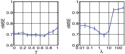
We also analyze parameter sensitivity, using the School dataset. Two key parameters in the proposed MTL-IRLS are γ and λ. The parameter λ controls the structure penalty, while γ plays a balancing role between group sparsity and element-wise sparsity. We use 30% data samples for training and the rest for testing. By fixing λ = 4 and varying γ in [0 : 0.1 : 1], we study how γ affects the performance. Similarly, we test the effect of λ by fixing γ = 0.5 and varying λ in 10i , i = -2 : 0.5 : 2.5. Figure 2 plots the regression performance measured by nMSE. We can observe that, with a fixed λ, the best performance of MTL-IRLS is obtained by setting γ to a value close to 0.5, which balances the effect of task grouping and task outlier. Overall the performance is quite stable for a fairly wide range of γ. However, when setting γ = 1 which only considers task outlier, the performance decreases dramatically, which further confirms that recovering the task group structure is more important than extracting outlier tasks. Finally, we notice that setting λ to be around 4 will produce the best results.
6 Conclusion
We have presented a novel MTL algorithm, namely MTLIRLS. Unlike several recent works that used a decomposition model, we directly imposed a regularization term with a mixture of structure and outlier penalties, which led to a flexible and robust formulation. To efficiently minimize the cost function, we proposed to use an Iteratively Reweighted Least Square method. We also provided a proof of convergence and discussed the performance bound. Experiments on both synthetic and real data have verified the effectiveness of MTL-IRLS, which offers consistently better performance than several state-of-the-art MTL algorithms. One interesting future work is to deploy MTL-IRLS in more challenging real-world applications.
Acknowledgments
This work was supported in part by two grants from the NSF China (#61201387 and #61228205), a National 973 Program (#2010CB327900), two grants from the STCSM (#12XD1400900 and #12511501602), and a New Teachers' Fund for Doctor Stations, Ministry of Education (#20120071120026), China.
@inproceedings{ijcai2013p239,
  title     = {Multiple Task Learning Using Iteratively Reweighted Least Square},
  author    = {Pu, Jian and Jiang, Yu-Gang and Wang, Jun and Xue, Xiangyang},
  booktitle = {Proceedings of the Twenty-Third International Joint Conference on
               Artificial Intelligence, {IJCAI-13}},
  publisher = {AAAI Press / International Joint Conferences on Artificial Intelligence},
  editor    = {Francesca Rossi},
  pages     = {1607--1612},
  year      = {2013},
  month     = {8},
  url       = {https://ijcai.org/proceedings/2013/239},
}
TY - CPAPER TI - Multiple Task Learning Using Iteratively Reweighted Least Square AU - Pu, Jian AU - Jiang, Yu-Gang AU - Wang, Jun AU - Xue, Xiangyang T2 - Proceedings of the Twenty-Third International Joint Conference on Artificial Intelligence, IJCAI-13 PB - AAAI Press / International Joint Conferences on Artificial Intelligence PY - 2013 SP - 1607 EP - 1612 UR - https://ijcai.org/proceedings/2013/239 ER -Copied
Machine-readable versions of this paper, for tools and AI agents:





