
Adaptive Loss Minimization for Semi-Supervised Elastic Embedding
Proceedings of the Twenty-Third International Joint Conference on Artificial Intelligence. Pages 1565-1570.
© 2013 International Joint Conferences on Artificial Intelligence
Abstract
The semi-supervised learning usually only predict labels for unlabeled data appearing in training data, and cannot effectively predict labels for testing data never appearing in training set. To handle this out-of-sample problem, many inductive methods make a constraint such that the predicted label matrix should be exactly equal to a linear model. In practice, this constraint is too rigid to capture the manifold structure of data. Motivated by this deficiency, we relax the rigid linear embedding constraint and propose to use an elastic embedding constraint on the predicted label matrix such that the manifold structure can be better explored. To solve our new objective and also a more general optimization problem, we study a novel adaptive loss with efficient optimization algorithm. Our new adaptive loss minimization method takes the advantages of both L1 norm and L2 norm, and is robust to the data outlier under Laplacian distribution and can efficiently learn the normal data under Gaussian distribution. Experiments have been performed on image classification tasks and our approach outperforms other state-of-the-art methods.
- [Belkin and Niyogi, 2003] M. Belkin and P. Niyogi. Lapla- cian eigenmaps for dimensionality reduction and data rep- resentation. Neural Computation, 15(6):1373-1396, 2003.
- [Belkin et al., 2006] Mikhail Belkin, Partha Niyogi, and Vikas Sindhwani. Manifold regularization: A geometric framework for learning from labeled and unlabeled ex- amples. Journal of Machine Learning Research, 7:2399- 2434, 2006.
- [Boyd and Vandenberghe, 2004] S.P. Boyd and L. Vanden- berghe. Convex optimization. Cambridge University Press, 2004.
- [Cai et al., 2011] Xiao Cai, Feiping Nie, Heng Huang, and Chris H. Q. Ding. Multi-class l2, 1-norm support vector machine. In ICDM, pages 91-100, 2011.
- [Ding et al., 2007] C. Ding, H.D. Simon, R. Jin, and T. Li. A learning framework using Green's function and kernel regularization with application to recommender system. In SIGKDD, 2007.
- [Ding, 2013] Chris Ding. A new robust function that smoothly interpolates between l1 and l2 error functions. Univerisity of Texas at Arlington Tech Report, 2013.
- [Gu and Zhou, 2009] Q. Gu and J. Zhou. Transductive clas- sification via dual regularization. In ECML/PKDD, 2009.
- [Joachims, 1999] Thorsten Joachims. Transductive inference for text classification using support vector machines. In ICML, pages 200-209, 1999.
- [Kondor and Lafferty, 2002] R.I. Kondor and J. Lafferty. Diffusion kernels on graphs and other discrete input spaces. In MACHINE LEARNING-INTERNATIONAL WORKSHOP THEN CONFERENCE-, pages 315-322, 2002.
- [Nie et al., 2010a] Feiping Nie, Heng Huang, Xiao Cai, and Chris Ding. Efficient and robust feature selection via joint ℓ 2,1 -norms minimization. In NIPS, 2010.
- [Nie et al., 2010b] Feiping Nie, Dong Xu, Ivor Wai-Hung Tsang, and Changshui Zhang. Flexible manifold embed- ding: A framework for semi-supervised and unsupervised dimension reduction. IEEE Transactions on Image Pro- cessing, 19(7):1921-1932, 2010.
- [Roweis and Al, 2000] Sam T. Roweis and Et Al. Nonlin- ear dimensionality reduction by locally linear embedding. Science, 290:2323-2326, 2000.
- [Szummer and Jaakkola, 2002] M. Szummer and T. Jaakkola. Partially labeled classification with Markov random walks. In NIPS, page 945, 2002.
- [Tenenbaum et al., 2000] J. B. Tenenbaum, V. de Silva, and J. C. Langford. A global geometric framework for nonlin- ear dimensionality reduction. Science, 290(5500):2319- 2323, December 2000.
- [Wang et al., 2011] H Wang, F Nie, H Huang, S L Risacher, C Ding, A J Saykin, L Shen, and ADNI. A new sparse multi-task regression and feature selection method to iden- tify brain imaging predictors for memory performance. ICCV 2011: IEEE Conference on Computer Vision, pages 557-562, 2011.
- [Xiang et al., 2009] Shiming Xiang, Feiping Nie, Changshui Zhang, and Chunxia Zhang. Nonlinear dimensionality re- duction with local spline embedding. IEEE Transactions on Knowledge and Data Engineering, 21(9):1285-1298, 2009.
- [Zhou et al., 2004] D. Zhou, O. Bousquet, T.N. Lal, J. We- ston, and B. Scholkopf. Learning with local and global consistency. In NIPS, page 321, 2004.
- [Zhu et al., 2003] Xiaojin Zhu, Zoubin Ghahramani, and John D. Lafferty. Semi-supervised learning using Gaus- sian fields and harmonic functions. In ICML, pages 912- 919, 2003.
References were extracted automatically from the PDF and may contain errors.
Full text extracted automatically from the PDF; figures, tables and equations may differ. The PDF is the version of record.
1 Introduction
In many real-world applications, because manually label data is expensive, we often have a small set of labeled data points together with a large collection of unlabeled data. Such a small size of labeled data inhabits the traditional supervised classification methods to achieve satisfied performance. To tackle this problem, in past ten years, the semi-supervised methods involving both labeled and unlabeled data to train classification model have attracted increasingly attention. Rather than discard the unlabeled outcomes during the training process, the semi-supervised learning methods attempt to extract information from the entire data set. The common assumption of semi-supervised learning methods is that if two input patterns are similar then their labels should also be similar. In the semi-supervised learning literature, this assumption is formulated by defining a similarity based adjacency graph over the unlabeled inputs and then defining a "smooth" function on the nodes such that, to the greatest extent possible, the function can assign neighboring nodes similar labels.
∗Corresponding Author. This work was partially supported by NSF CCF-0830780, CCF-0917274, DMS-0915228, IIS-1117965.
Based on this assumption, many semi-supervised learning methods have been proposed to utilize the label propagation from labeled data to unlabeled data on the adjacency graph. In its simplest form, the label propagation is like a random walk on the adjacency graph [Szummer and Jaakkola, 2002]. Using the diffusion kernel, the semi-supervised learning is like a diffusive process of the labeled information [Kondor and Lafferty, 2002]. The harmonic function approach [Zhu et al., 2003] emphasizes the harmonic nature of the diffusive function. The consistency labeling approach [Zhou et al., 2004] focuses on the spread of label information in an iterative way.
The success of semi-supervised learning is based on how much information unlabeled data carry about the distribution of labels in the pattern space. To enhance the strength of semi-supervise learning models, two challenges should be addressed: 1) how to make an out-of-sample predication, i.e., to classify an input data which is not a node of the graph defined by the unlabeled training data; 2) how to efficiently handle the data with high-dimensional features, such as the images, videos, and biological data. In general, researchers hypothesize a low-dimensional manifold structure along which labels can be assumed to vary smoothly [Belkin et al., 2006]. To discover the intrinsic manifold structure of the data, many nonlinear dimension reduction algorithms have been proposed, such as Isomap [Tenenbaum et al., 2000], Locally Linear Embedding (LLE) [Roweis and Al, 2000], Laplacian Eigenmap [Belkin and Niyogi, 2003] and Local Spline Embedding (LSE) [Xiang et al., 2009]. However, these methods suffer from the out-of-sample problem. Because the linear models are efficient in learning process and have good empirical performance, the linear manifold regularization was introduced to semi-supervised learning to solve both out-of-sample and dimension reduction problems [Belkin et al., 2006]. In this model, a linear discriminator in a predefined vector space was introduced to handle out-ofsample inputs. However, the rigid linear embedding used in such semi-supervised learning model often restricts the identification of manifold structure and reduces the classification performance of semi-supervised learning.
To solve these problems, inspired by [Nie et al., 2010b], we propose a new elastic embedding constraint on the predicted label matrix such that the manifold structure can be better explored and a linear model is also learned for induction. Moreover, we study a novel adaptive loss with efficient optimization algorithm, which can solve the proposed objective and also tackle the more general problem. Our new adaptive loss can model the objective function to be robust to the data outlier (under Laplacian distribution) and be efficient in learning from the normal data (under Gaussian distribution). Experiments have been performed on image classification problem to evaluate the new method. In all empirical results, our approach outperforms other state-of-the-art methods.
2 Semi-Supervised Learning with Elastic Embedding
2.1 RelatedWork
Given n training data points {x1, x2, ..., xn}, denote the data matrix X = [x1, x2, ..., xn] ∈ Rd×n , where d is the dimensionality. In the graph based method, a graph is constructed based on the training data points and a similarity matrix A ∈ Rn×n associated with the graph is calculated to encode the similarities between data pairs. The Laplacian matrix on the graph is defined as L = D-A, where D is the diagonal matrix with the i-th diagonal element Dii = ∑i Aij .
In the semi-supervised learning methods, the training data include only a few data points with labels, and the remaining training data points are unlabeled. Without loss of generality, suppose the first l data points x1, x2, ..., xl are labeled and the data points xl+1, xl+2, ..., xn are unlabeled. For simplicity and easy reading, we first discuss the binary class case and then introduce how to extend to multiple class case. Suppose the labels of the first l data points are y1, y2, ..., yl, respectively. For each i, yi ∈ {-1,+1}. The task of semisupervised learning is to predict the labels for the unlabeled data points and new coming data points. Denote the label vector of the first l data points by y(l) ∈ Rl×1 , where the (i)- th element of y(l) is yi. Denote the predicted label vector by
Recently, manifold regularization method was proposed to perform inductive (handling both the in-sample and out-ofsample data) semi-supervised learning, which is to solve the following problem:
where Xl = [x1, x2, ..., xl] ∈ Rd×l . The basic idea of this inductive method is to learn a linear model by constraining XT w + 1b = f, where w is the projection vector, b is the bias scatter, 1 is a vector with all the elements as one.
2.2 Semi-Supervised Elastic Embedding
As can be seen in Eq. (1), the manifold regularization method made a constraint that the predicted label matrix f must be exactly equal to the linear model XT w+1b. In practice, this constraint XT w + 1b = f might be too rigid to capture the manifold structure of data for label propagation. Inspired by [Nie et al., 2010b], in this paper we propose to use an elastic term ∥∥XT w + 1b - f ∥∥22 to better explore the manifold structure of data and also to learn a linear model for induction. Note that the classic linear model ∥∥XT w+ 1b - y∥∥22 (y is the given labels of labeled data) is often used for classification, the f in the elastic term is the predicted labels of both labeled and unlabeled data. In practice, labeled data are usually few and we can make a reasonable assumption that all the labels of the labeled data are correct, so f(l) = y(l). For these reasons, we propose to use an elastic embedding to solve the following problem:
Note that in the elastic embedding, since all the training data are used to learning the projection w, we do not add the regularization term ‖w‖22 to avoid overfitting as in Eq. (1). Experimental results show this elastic embedding model performs well without the regularization, thus reduces the burden of parameter tuning, which is usually a difficult task in practices.
Interestingly, there is closed form optimal solution to Eq. (2). By setting the derivative of Eq. (2) w.r.t. b to 0, we have
Substituting into Eq. (2), and by setting the derivative of Eq. (2) w.r.t. W to 0, we have 1
where C = I - 1n 11T is the centering matrix. Again substituting into Eq. (2), we have
Then the optimal solution f(u) is
where
2.3 Multi-Class Extension
In the multi-class case, the label matrix should be redefined. As before, suppose the first l data points x1, · · · , xl are labeled. Denote the label matrix of the first l data points by Y(l) ∈ Rl×c , where the (i, j)-th element of Y(l) is 1 if xi is labeled as class j and 0 otherwise. Denote the predicted
1 Note that X is the total training data matrix, the null space of the training data should be removed before learning a linear model, so XCXT is invertible.
Extending the graph based methods from binary class to multi-class is usually very easy. For example, the binary elastic embedding model in Eq. (2) can be extended to the multiclass case by solving the following problem:
Similarly to the problem (2), there is also a closed form optimal solution to Eq. (7).
3 Semi-Supervised Elastic Embedding with Adaptive Loss Minimization
In practice, unlabeled data are often very abundant, and usually there are some outliers in the unlabeled data. It is known that the traditional squared L2-norm loss is sensitive to outliers. In this paper, we study a recently proposed adaptive loss[Ding, 2013] which is not sensitive to outliers , then we apply this loss function in the elastic embedding model.
3.1 Adaptive Loss Function of Vector
For a vector x, traditional L1-norm and squared L2-norm are defined by ‖x‖1 = ∑i |xi| and ‖x‖22 = ∑i x2i , respectively.
Using squared L2-norm as loss function is not sensitive to small loss but is sensitive to outliers, outliers with large loss will dominate the objective function and thus impose great impact on the model learning. Although using L1-norm as loss function is not sensitive to outliers, it is sensitive to small loss (penalizes more for the small loss than L2-norm does). In general, given a correct model, most data should have small loss to fit the model, and only a few data have large loss to fit the model, which can be seen as outlier under this model. The small loss of most data can be reasonably assumed to be Gaussian (normal) distribution, while the large loss of a few data can be reasonably assumed to be Laplacian distribution. Based on this motivation, we define an adaptive loss function of vector in the model learning.
Given a vector x, the adaptive loss function [Ding, 2013] is defined as
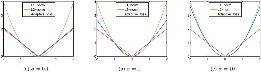
where xi is the i-th element of the vector x and σ is an adaptive parameter of the loss function. This function smoothly interpolates between L1-norm and L2-norm. The comparison of L1-norm, L2-norm and the adaptive loss function with different σ is illustrated in Fig 1. This loss function has the following interesting properties:
1. ‖x‖σ is nonnegative and convex, which is desirable for a loss function.
- ‖x‖σ is twice differentiable, which is desirable for optimization.
- When ∀i, xi ≪ σ, then ‖x‖σ → (1+σ) σ ‖x‖22 .
- When ∀i, xi ≫ σ, then ‖x‖σ → (1 + σ) ‖x‖1 .
- When σ → 0, then ‖x‖σ → ‖x‖1 .
- When σ → ∞, then ‖x‖σ → ‖x‖22 .
In this paper, we apply the adaptive loss function in the elastic embedding model, which is to solve the following problem:
The problem (9) is convex and differentiable, we will propose an effective algorithm to find the optimal solution.
3.2 Adaptive Loss Function of Matrix
We extend the adaptive loss function for vector to the adaptive loss function for matrix. For a matrix X, traditional L21norm and squared F-norm are defined by ‖X‖2,1 = ∑i ∥∥xi∥∥2
and ‖X‖2F = ∑i ∥∥xi∥∥22 respectively, where xi denotes the i-th row of matrix X.
Given a matrix X, the proposed adaptive loss function is defined as
One can see when X reduced to a vector, Eq. (10) reduced to Eq. (8).
Similarly, this loss function also has the following interesting properties:
1. ‖X‖σ is nonnegative and convex, which is desirable for a loss function.
2. ‖X‖σ is twice differentiable, which is desirable for optimization.
- When ∀i, ∥∥xi∥∥2 ≪ σ, then ‖X‖σ → (1+σ) σ ‖X‖2F .
- When ∀i, ∥∥xi∥∥2 ≫ σ, then ‖X‖σ → (1 + σ) ‖X‖2,1 .
- When σ → 0, then ‖X‖σ → ‖X‖2,1 .
- When σ → ∞, then ‖X‖σ → ‖X‖2F .
In this paper, we apply the adaptive loss function in the elastic embedding model, which is to solve the following problem:
The problem (11) is convex and differentiable, we will propose an effective algorithm to find the optimal solution in the next section.
4 Optimization Algorithm
4.1 Algorithm for AMore General Adaptive Loss Minimization Problem
First, let us consider a more general adaptive loss minimization problem as follows:
where gi(x) is a vector or matrix output function. It can be seen that the problem (9) and (11) are special case of the problem (12). Based on our previous sparse learning optimization algorithms [Nie et al., 2010a; Cai et al., 2011; Wang et al., 2011], we propose an iteratively re-weighted method to solve problem (12).
Algorithm 1 Algorithm to solve the problem (12).
Guess x.
repeat
until Converges
By setting the derivative of Eq. (12) w.r.t. x to zero, we have
Denote
Then Eq. (13) is rewritten as
Note that di is dependent on x, this equation is difficult to solve. However, if di is given for every i, then solving Eq. (15) is equivalent to solving the following problem:
Based on the above analysis, we propose an iterative algorithm to find the solution of Eq. (13), and thus the optimal solution of problem (12). We will give a theoretical analysis to prove the convergence of the proposed algorithm. The detailed algorithm is described in Algorithm 1. In the algorithm, We first guess a solution x, then we calculate di based on the current solution x and update the current solution x by the optimal solution of problem (16) based on the calculated si, this procedure is iteratively performed until converges.
4.2 Convergence Analysis of Algorithm 1
To prove the convergence of the Algorithm 1, we need the following lemma:
Lemma 1 For any vectors x, y with the same size, the following inequality holds:
Proof:
which completes the proof.
□
As a result, we have the following theorem:
Theorem 1 The Algorithm 1 will monotonically decrease the objective of the problem (12) in each iteration.
Proof: In step 2 of Algorithm 1, suppose the updated x is ˜x. According to step 2, we know that
Note that di = (1 + σ) ‖gi(x)‖2+2σ 2(‖gi(x)‖2+σ)2 , so we have
According to Lemma 1, we have
Summing Eq. (18) and Eq. (19) in the two sides, we arrive at
Thus the Algorithm 1 will monotonically decrease the objective of the problem (12) in each iteration until the algorithm converges. □
In the convergence, the equality in Eq. (13) holds, thus the KKT condition [Boyd and Vandenberghe, 2004] of problem (12) is satisfied. Therefore, the Algorithm 1 will converge to an optimum solution to the problem (12).
4.3 Optimization Algorithm to Problem of Eq. (11)
In this subsection, we describe how to solve the problem (11) based on the Algorithm 1. According to the step 2 in Algorithm 1, i.e. Eq. (16), the key step of solving problem (11) is to solve the following problem:
where D is a diagonal matrix with the i-th diagonal element di = (1 + σ) ‖xTi W+bT -f i ‖2+2σ
By setting the derivative of Eq. (20) w.r.t. b to 0, we have
Substituting into Eq. (20), and by setting the derivative of Eq. (20) w.r.t. W to 0, we have
where N = D - 1 1T D1 D11T D is the centering matrix. Again substituting into Eq. (20), we have
(23)
Then the optimal solution f(u) is
where
Based on the above analysis, we propose an iterative algorithm to solve the problem (11). The detailed algorithm is described in Algorithm 2. The algorithm will converge to the optimal solution according to Theorem 1.
Algorithm 2 Algorithm to solve the problem (11).
Guess W, b, F .
repeat
- Calculate a diagonal matrix D with the i-th diagonal element di = (1 + σ) ‖xTi W+bT -f i ‖2+2σ 2(‖xTi W+bT -f i ‖2+σ)2
- Update F by Eq. (24), update W by Eq. (22), Update b by Eq. (21).
until Converges
5 Experiments
5.1 Implementation Details of Our Method
Parameter selection. The proposed method has two parameters γ and σ in Eq. (11). The parameter γ balances the manifold regularization and the proposed new loss function. For simplicity, we set γ = 1 in all our experiments. The parameter σ controls the property of our new loss function: when σ → ∞, our new loss function is equivalent to squared ℓ2norm loss function; and when σ → 0, our new loss function is equivalent to ℓ1-norm loss function. Therefore, we can reasonably select σ in the range of [0,+∞). Upon our preliminary experiments, we empirically set σ = 0.1 in our experiments.
Classification rule. Given the output decision matrix F from Algorithm 2 for both labeled and unlabeled data points, their relevances to the classes of interest are ranked, upon which we can assign labels to the unlabeled data points: we classify an unlabeled data point xi (l + 1 ≤ i ≤ n) by the following rule: l (xi) = argmaxk Fik.
For the classification of an out-of-sample data point x ∈ Rd , we first compute its decision vector by f = W T x + b, where W is the output projection matrix and b is output bias vector from Algorithm 2. Then we predict labels for x by applying the same classification rules as above.
5.2 Improved Classification Results
We evaluate the capability of the proposed method in classification tasks. We experiment with the following two data sets Caltech-101 2 and MSRC-v1 3 for four image classification tasks, which are broadly used as benchmark in both computer vision and machine learning studies.
For our method, besides implementing the one defined in Eq. (11) using the new loss function, denoted as "SEE", we also implements the version using least square loss function which is defined in Eq. (7) and denoted as "SEE-LS".
Image feature extraction. We divide each image into 64 blocks by a 8 × 8 grid and compute the first and second moments (mean and variance) of each color band in the Lab color space to obtain a 384-dimensional feature vector. Other features can also be used for our method.
Experimental setups. We compare our method against its most related method, i.elet@tokeneonedot, the LapRLS
2 http://www.vision.caltech.edu/Image Datasets/Caltech101/
3 http://research.microsoft.com/enus/projects/objectclassrecognition/
| Methods | Caltech-7 classes | Caltech-20 classes | Caltech-all classes | MSRC-v1 |
|---|---|---|---|---|
| SVM TSVM GFHF GF SEE SVM TSVM GFHF GF | 0.75 ±0.15 | 0.50 ±0.17 | 0.37±0.12 | 0.76±0.20 |
| 0.81 ±0.04 | 0.56 ±0.04 | 0.41±0.03 | 0.78±0.06 | |
| 0.51 ±0.09 | 0.38 ±0.07 | 0.21±0.04 | 0.56±0.09 | |
| 0.63 ±0.06 | 0.42±0.03 | 0.26±0.02 | 0.60± 0.06 | |
| TCDR | 0.81 ±0.09 | 0.62±0.04 | 0.51±0.07 | 0.82±0.07 |
| LapRLS | 0.77 ±0.09 | 0.49±0.12 | 0.40±0.05 | 0.74±0.06 |
| SEE-LS | 0.82 ±0.04 | 0.65±0.03 | 0.57±0.04 | 0.86±0.02 |
| 0.86±0.05 | 0.70±0.02 | 0.63±0.04 | 0.89±0.04 | |
| 0.51 ±0.12 | 0.33 ±0.14 | 0.25±0.14 | 0.51±0.16 | |
| 0.63 ±0.03 | 0.44 ±0.04 | 0.32±0.04 | 0.63±0.05 | |
| 0.40 ±0.07 | 0.31 ±0.08 | 0.18±0.03 | 0.45±0.07 | |
| 0.51 ±0.05 | 0.34±0.04 | 0.21±0.04 | 0.48± 0.05 | |
| TCDR | 0.64 ±0.08 | 0.50±0.06 | 0.41±0.05 | 0.65±0.06 |
| LapRLS | 0.53 ±0.07 | 0.36±0.10 | 0.27±0.07 | 0.52±0.08 |
| SEE-LS | 0.71 ±0.05 | 0.56±0.04 | 0.49±0.05 | 0.74±0.04 |
| SEE | 0.78±0.06 | 0.64±0.04 | 0.57±0.03 | 0.81±0.05 |
method as defined in Eq. (1). We also compare our method to the following widely used semi-supervised method including Transductive SVM (TSVM) [Joachims, 1999] method, Gaussian Field and Harmonic function (GFHF) [Zhu et al., 2003] method, Green's Function (GF) [Ding et al., 2007] method and Transductive Classification via Dual Regularization (TCDR) [Gu and Zhou, 2009] method. As a baseline, we also report the classification performances of SVM on the same data sets, though it is a supervised classification method. We implement SVM and TSVM methods using the SVMlight software package 4 . Following [Joachims, 1999], we fix the regularization parameter C = 1 and use the Gaussian kernel (i.elet@tokeneonedot, K(xi, xj) = exp (-γ ‖xi -xj‖2)) where γ is fined tuned in the range of {10-5 , . . . , 10-1 , 1, 101 , . . . , 105}. For SVM and TSVM methods, we employ one-vs-other strategy to deal with multiclass data sets. We implement the other compared methods and set the parameters to be optimal following their original works.
Experimental results. For each of the four classification tasks from the two image data sets, we randomly select 20% images as labeled data and the rest as unlabeled data, on which we perform all the compared methods. A 5-fold crossvalidation is conducted on the labeled data to fine tune the parameters of the compared methods. We repeat each test case for 20 times and report the average performance. Because we experiment with single-label data, the macro average classification accuracies over all the classes of the compared methods are reported in the top half of Table 1, from which we have a number of interesting observations as following.
First, the proposed methods are consistently better than the compared methods with a significant margin, which clearly demonstrate their effectiveness in classification. Moreover, the proposed SEE method always outperforms its variant of SEE-LS method, which shows that the proposed new loss function is better for classification tasks.
4 http://svmlight.joachims.org/
Second, our new methods obviously outperform their nonrobust and rigid counterpart, i.e., the LapRLS method, which is consistent with our previous theoretical analyses: our method does better in the robustness against noises and outlier samples that are inevitable in large-scale data and its elasticity between the predicted and ground truth labels for the labeled data. These important results concretely confirm the correctness and advantage of our learning objective in Eq. (11) over that of the LapRLS method in Eq. (1).
Last, but not least, the performance perturbation measured by standard deviation of the SVM method is considerably greater than those of the other six compared semi-supervised learning methods including ours. This is because in our experiments the amount of the labeled data (20%) is much smaller that of unlabeled data (80%), which is the standard semi-supervised learning setting and the settings of many real world applications. As a result, supervised learning method such as SVM can only use the labeled data but not able to take advantage of the valuable information contained in the large amount of unlabeled data, which thus demonstrate the practical use of the semi-supervised learning methods such as the proposed one.
5.3 Robustness of Our Methods Against Noise
Because an important advantage of the proposed new loss function defined in Eq. (11) lies in its robustness against noise, in this subsection we further evaluate the classification capability of the proposed methods in semi-supervised learning on noisy data, where we use the same data and experimental settings as the previous subsection with the following change. We randomly select 50% of training data in each trial of every experiment and assign incorrect class labels to them to emulate noise.
The classification results of the compared methods are reported in the bottom half of Table 1. A first glance at the results show that our methods are still better than the competing methods. A more careful analysis on the results show that, although the classification performances of our methods are not as good as those on the noiseless data, their degradations are much smaller than those of other compared methods. From these observations we can conclude the superiority of our newmethods in their robustness against noise.
6 Conclusions
In this paper, a semi-supervised elastic embedding constraint and a novel adaptive loss minimization method were proposed. To handle the out-of-sample problem in transductive semi-supervised learning, we relax the rigid linear model constraint by an elastic constraint such that the manifold structure can be better explored. Furthermore, we study a novel adaptive loss minimization method with efficient algorithm and rigorously proved convergence. Experimental results on image categorizations clearly show the effectiveness of the proposed method.
@inproceedings{ijcai2013p233,
  title     = {Adaptive Loss Minimization for Semi-Supervised Elastic Embedding},
  author    = {Nie, Feiping and Wang, Hua and Huang, Heng and Ding, Chris H. Q.},
  booktitle = {Proceedings of the Twenty-Third International Joint Conference on
               Artificial Intelligence, {IJCAI-13}},
  publisher = {AAAI Press / International Joint Conferences on Artificial Intelligence},
  editor    = {Francesca Rossi},
  pages     = {1565--1570},
  year      = {2013},
  month     = {8},
  url       = {https://ijcai.org/proceedings/2013/233},
}
TY - CPAPER TI - Adaptive Loss Minimization for Semi-Supervised Elastic Embedding AU - Nie, Feiping AU - Wang, Hua AU - Huang, Heng AU - Ding, Chris H. Q. T2 - Proceedings of the Twenty-Third International Joint Conference on Artificial Intelligence, IJCAI-13 PB - AAAI Press / International Joint Conferences on Artificial Intelligence PY - 2013 SP - 1565 EP - 1570 UR - https://ijcai.org/proceedings/2013/233 ER -Copied
Machine-readable versions of this paper, for tools and AI agents:





