Learning Canonical Correlations of Paired Tensor Sets Via Tensor-to-Vector Projection

1 Introduction

Canonical correlation analysis (CCA) [Hotelling, 1936] is a well-known method for analyzing the relations between two sets of vector-valued variables. It assumes that the two data sets are two views of the same set of objects and projects them into low dimensional spaces where each pair is maximally correlated subject to being uncorrelated with other pairs. CCA has various applications such as information retrieval [Hardoon et al., 2004], multi-label learning [Sun et al., 2008; Rai and Daum´e III, 2009] and multi-view learning [Chaudhuri et al., 2009; Dhillon et al., 2011].

Many real-world data are multi-dimensional, represented as tensors rather than vectors. The number of dimensions is the order of a tensor. Each dimension is a mode. Secondorder tensors include matrix data such as 2-D images. Examples of third-order tensors are video sequences, 3-D images, and web graph mining data organized in three modes of source, destination and text [Kolda and Bader, 2009; Kolda and Sun, 2008].

To deal with multi-dimensional data effectively, researchers have attempted to learn features directly from tensors [He et al., 2005]. The motivation is to preserve data structure in feature extraction, obtain more compact representation, and process big data more efficiently, without reshaping tensors into vectors. Many multilinear subspace learning (MSL) algorithms [Lu et al., 2011] generalize linear algorithms such as principal component analysis and linear discriminant analysis to second/higher-order [Ye et al., 2004a; 2004b; Yan et al., 2005; Tao et al., 2007; Lu et al., 2008; 2009a; 2009b]. There have also been efforts to generalize CCA to tensor data. To the best of our knowledge, there are two approaches.

One approach analyzes the relationship between two tensor data sets rather than vector data sets. The two-dimensional CCA (2D-CCA) [Lee and Choi, 2007] is the first work along this line to analyze relations between two sets of image data without reshaping into vectors. It was further extended to local 2D-CCA [Wang, 2010], sparse 2D-CCA [Yan et al., 2012], and 3-D CCA (3D-CCA) [Gang et al., 2011]. Under the MSL framework, these CCA extensions are using the tensor-to-tensor projection (TTP) [Lu et al., 2011].

Another approach studies the correlations between two data tensors with one or more shared modes because CCA can be viewed as taking two data matrices as input. This idea was first introduced in [Harshman, 2006]. Tensor CCA (TCCA) [Kim and Cipolla, 2009] was proposed later with two architectures for matching (3-D) video volume data of the same dimensions. The single-shared-mode and joint-sharedmode TCCAs can be viewed as transposed versions of 2DCCA and classical CCA, respectively. They apply canonical transformations to the non-shared one/two axes of 3-D data, which can be considered as partial TTPs under MSL. Following TCCA, the multiway CCA in [Zhang et al., 2011] uses partial projections to find correlations between second-order and third-order tensors.

However, none of the multilinear extensions above takes an important property of CCA into account, i.e., CCA extracts uncorrelated features for different pairs of projections. To close this gap, we propose a multilinear CCA (MCCA) algorithm for learning canonical correlations of paired tensor data sets with uncorrelated features under two architectures. It belongs to the first approach mentioned above.

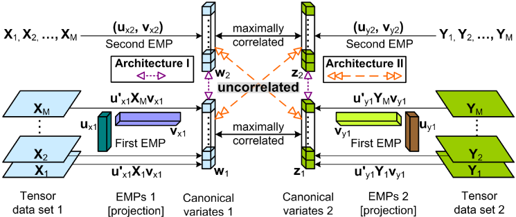
MCCA uses the tensor-to-vector projection (TVP) [Lu et al., 2009a], which will be briefly reviewed in Sec. 2. We follow the CCA derivation in [Anderson, 2003] to successively solve for elementary multilinear projections (EMPs) to maximize pairwise correlations while enforcing same-set or crossset zero-correlation constraint in Sec. 3. Finally, we evaluate the performance on facial image matching in Sec. 4.

To reduce notation complexity, we present our work here only for second-order tensors, i.e., matrices, as a special case, although we have developed MCCA for general tensors of any order following [Lu et al., 2011].

2 Preliminary of CCA and TVP

2.1 CCA and zero-correlation constraint

CCA captures the correlations between two sets of vectorvalued variables that are assumed to be different representations of the same set of objects [Hotelling, 1936]. For two paired data sets xm ∈ RI , ym ∈ RJ , m = 1, ..., M, I ̸= J in general, CCA finds paired projections {uxp , uyp }, uxp ∈ RI , uyp ∈ RJ , p = 1, ..., P, such that the canonical variates wp and zp are maximally correlated. The mth elements of wp and zp are denoted as wpm and zpm , respectively:

where u′ denotes the transpose of u. In addition, for p ̸= q (p, q = 1, ..., P), wp and wq, zp and zq, and wp and zq, respectively, are all uncorrelated. Thus, CCA produces uncorrelated features both within each set and between different pairs of the two sets.

The solutions {uxp , uyp } for this CCA problem can be obtained as eigenvectors of two related eigenvalue problems. However, a straightforward generalization of these results to tensors [Lee and Choi, 2007; Gang et al., 2011] does not give uncorrelated features while maximizing the paired correlations (to be shown in Figs. 3(b) and 3(c)). Therefore, we derive MCCA following the more principled approach of solving CCA in [Anderson, 2003], where CCA projection pairs are obtained successively through enforcing the zerocorrelation constraints.

2.2 TVP: tensor space to vector subspace

To extract uncorrelated features from tensor data directly, we use the TVP in [Lu et al., 2009a]. The TVP of a matrix X ∈ RI1×I2 to a vector r ∈ RP consists of P EMPs {up, vp}, up ∈ RI1 , vp ∈ RI2 , p = 1, ..., P. It is a mapping from the original tensor space RI1 ⊗ RI2 into a vector subspace RP . The pth EMP (up, vp) projects X to a scalar rp, the pth element of r, as:

Define two matrices U = [u1, ..., uP ] ∈ RI1×P and V = [v1, ..., vP ] ∈ RI2×P , then we have

where diag(·) denotes the main diagonal of a matrix.

3 Multilinear CCA

This section proposes MCCA for analyzing the correlations between two matrix data sets by first formulating the problem, and then adopting the successive maximization approach [Anderson, 2003] and alternating projection method [Lu et al., 2011] to solve it.

3.1 Problem formulation through TVP

In (second-order) MCCA, we consider two matrix data sets with M samples each: {Xm ∈ RI1×I2 } and {Ym ∈ RJ1×J2 }, m = 1, ...,M. I1 and I2 may not equal to J1 and J2, respectively. We assume that their means have been subtracted so that they have zero-mean, i.e., ∑Mm=1 Xm = 0 and ∑Mm=1 Ym = 0. We are interested in paired projections {(uxp , vxp ), (uyp , vyp )}, uxp ∈ RI1 , vxp ∈ RI2 , uyp ∈ RJ1 , vyp ∈ RJ2 , p = 1, ..., P , for dimensionality reduction to vector spaces to reveal correlations between them. The P projection pairs form matrices Ux = [ux1 , ..., uxP ], Vx = [vx1 , ..., vxP ], Uy = [uy1 , ..., uyP ], and Vy = [vy1 , ..., vyP ]. The matrix sets {Xm} and {Ym} are projected to {rm ∈ RP } and {sm ∈ RP }, respectively, through TVP (3) as

We can write the projection above according to EMP (2) as

where rmp and smp are the pth elements of rm and sm, respectively. We then define two coordinate vectors wp ∈ RM and zp ∈ RM for the pth EMP, where their pth elements wpm = rmp and zpm = smp . Denote R = [r1, ..., rM], S = [s1, ..., sM], W = [w1, ...,wP ], and Z = [z1, ..., zP ]. We have W = R′ and Z = S′ . Here, wp and zp are analogous to the canonical variates in CCA [Anderson, 2003].

We propose MCCA with two architectures. Architecture I: wp and zp are maximally correlated, while for q ̸= p (p, q = 1, ..., P), wq and wp, and zq and zp, respectively, are uncorrelated. Architecture II: wp and zp are maximally correlated, while for q ̸= p (p, q = 1, ..., P), wp and zq are uncorrelated. Figure 1 is a schematic diagram showing MCCA and its two different architectures.

We extend the sample-based estimation of canonical correlations and variates in CCA to the multilinear case for matrix data using Architecture I.

Definition 1. Canonical correlations and variates for matrix data (Architecture I). For two matrix data sets with M samples each {Xm ∈ RI1×I2 } and {Ym ∈ RJ1×J2 }, m = 1, ...,M, the pth pair of canonical variates is the pair {wpm = u′xp Xmvxp } and {zpm = u′yp Ymvyp }, where wp and zp have maximum correlation ρp while for q ̸= p (p, q = 1, ..., P ), wq and wp, and zq and zp, respectively, are uncorrelated. The correlation ρp is the pth canonical correlation.

An analogous definition with Architecture II follows by changing the constraint accordingly.

3.2 Successive derivation of MCCA algorithm

Here, we derive MCCA with Architecture I (MCCA1). MCCA with Architecture II (MCCA2) differs fromMCCA1 only in the constraints enforced so it can be obtained in an analogous way by swapping wq and zq (q = 1, ..., p - 1) below. Following the successive derivation of CCA in [Anderson, 2003], we consider the canonical correlations one by one. The MCCA objective function for the pth EMP pair is

where the sample Pearson correlation coefficient ρp between wp and zp is given by 1 :

The P EMP pairs in the MCCA problem are determined one pair at a time in P steps, with the pth step obtaining the pth EMP pair:

Step 1: Determine {(ux1 , vx1 ), (uy1 , vy1 )} that maximizes ρ1 without any constraint.

To solve for the pth EMP pair, we need to determine four projection vectors, uxp , vxp , uyp , and vyp . As their simultaneous determination is difficult, we follow the alternating projection method [Lu et al., 2011] derived from alternating least squares [Harshman, 1970]. To determine each EMP pair, we estimate uxp and uyp conditioned on vxp and vyp first, then we estimate vxp and vyp conditioned on uxp and uyp .

Conditional subproblem: To estimate uxp and uyp conditioned on vxp and vyp , we assume that vxp and vyp are given and they can project input samples to obtain vectors

The conditional subproblem then becomes to determine uxp and uyp that project the samples {˜rmp } and {˜smp } (m =

1 Note that the means of wp and zp are both zero since the input matrix sets are assumed to be zero-mean.

1, ...,M) to maximize their correlation subject to the zerocorrelation constraint, which is a CCA problem with input samples {˜rmp } and {˜smp }.

The corresponding maximum likelihood estimator of the covariance matrices are defined as [Anderson, 2003]

where ˜Σrsp = ˜Σ′srp .

For p = 1, we solve for ux1 and uy1 that maximize the correlation between the projections of {˜rmp } and {˜smp } without any constraint. We get ux1 and uy1 as the leading eigenvectors of the following eigenvalue problems as in CCA [Hardoon et al., 2004; Dhillon et al., 2011]:

where we assume that ˜Σssp and ˜Σrrp are nonsingular throughout this paper.

Constrained optimization for p > 1: Next, we determine the pth (p > 1) EMP pair given the first (p-1) EMP pairs by maximizing the correlation ρp, subject to the constraint that features projected by the pth EMP pair are uncorrelated with those projected by the first (p - 1) EMP pairs. Due to the fundamental difference between linear and multilinear projections, the remaining eigenvectors of (11) and (12), which are the solutions of CCA for p > 1, are not the solutions for our MCCA problem. Instead, we have to solve a new constrained optimization problem in the multilinear setting.

Let ˜Rp ∈ RI1×M and ˜Sp ∈ RJ1×M be matrices with ˜rmp and ˜smp as their mth columns, respectively, i.e.,

then the pth coordinate vectors are wp = ˜R′puxp and zp = ˜S′puyp . The constraint that wp and zp are uncorrelated with {wq} and {zq}, respectively, can be written as

The coordinate matrices are formed as

Thus, we determine uxp and uyp (p > 1) by solving the following constrained optimization problem:

where the pth (sample) canonical correlation

The solution is given by the following theorem:

Theorem 1. For nonsingular ˜Σrrp and ˜Σssp , the solutions for uxp and uyp in the problem (17) are the eigenvectors corresponding to the largest eigenvalue λ of the following eigenvalue problems:

and I is an identity matrix.

Proof. For nonsingular ˜Σrrp and ˜Σssp , any uxp and uyp can be normalized such that u′xp ˜Σrrp uxp = u′yp ˜Σssp uyp = 1 and the ratio ˜ ρp keeps unchanged. Therefore, maximizing ˜ ρp is equivalent to maximizing u′xp ˜Σrsp uyp with these normalization constraints. Lagrange multipliers can be used to transform the problem (17) to the following to include all the constraints:

where where φ, ψ, {θq}, and {ωq} are Lagrange multipliers. Let θp-1 = [θ1 θ2 ... θp-1]′ , ωp-1 = [ω1 ω2 ... ωp-1]′ , then we have the two summations in (25) as ∑p-1 q=1 θq ˜Rpwq =

The vectors of partial derivatives of ϕp with respect to the elements of uxp and uyp are set equal to zeros, giving

Multiplication of (26) on the left by u′xp and (27) on the left by u′yp results in

Since u′xp ˜Σrrp uxp = 1 and u′yp ˜Σssp uyp = 1, this shows that φ = ψ = u′xp ˜Σrsp uyp .

Next, we have the following using the definitions in (23) and (24) through multiplication of (26) on the left by W′p-1 ˜R′p ˜Σ-1 rrp and (27) on the left by Z′p-1 ˜S′p ˜Σ-1 ssp :

Solving for θp-1 from (30) and ωp-1 from (31), and substituting them into (26) and (27), we have the following based on earlier result φ = ψ and the definitions in (21) and (22):

Let λ = φ2 (then φ = √λ), we have two eigenvalue problems in (19) and (20) from (32). Since φ(= √λ) is the criterion to be maximized, the maximization is achieved by setting uxp and uyp to be the eigenvectors corresponding to the largest eigenvalue of (19) and (20), respectively.

By setting Φ1 = I, Ψ1 = I, we can write (11) and (12) in the form of (19) and (20) as well. In this way, (19) and (20) give unified solutions for {(uxp , vxp ), (uyp , vyp )}, p = 1, ..., P . They are unique only up to sign [Anderson, 2003].

Similarly, to estimate vxp and vyp conditioned on uxp and uyp , we project input samples to obtain

This conditional subproblem can be solved similarly by following the derivation from (9) to (24). Algorithm 1 summarizes the MCCA algorithm for Architecture I 2 . For simplicity and reproducibility, we adopt the uniform initialization scheme in [Lu et al., 2009b] where each vector is initialized to all ones vector 1 and then normalized to unit vector. The iteration is terminated by setting a maximum iteration number K for computational efficiency.

2 The MATLAB code for MCCA will be made available at: http: //www.mathworks.com/matlabcentral/fileexchange/authors/80417

Algorithm 1 Multilinear CCA for matrix sets (Arch. I)

• 1: Input: Two zero-mean matrix sets: {Xm ∈ RI1×I2 } and {Ym ∈ RJ1×J2 }, m = 1, ...,M, the subspace dimension P , and the maximum number of iterations K.
• 2: for p = 1 to P do
• 3: Initialize vxp(0) = 1/ ‖ 1 ‖, vyp(0) = 1/ ‖ 1 ‖.
• 4: for k = 1 to K do
• 5: Mode 1:
• 6: Calculate {˜rmp } and {˜smp } according to (8) with vxp(k-1) and vyp(k-1) for m= 1, ...,M.
• 7: Calculate ˜Σrrp , ˜Σssp , ˜Σrsp and ˜Σsrp from (9) and (10).
• 8: Form ˜Rp and ˜Sp according to (13).
• 9: Calculate Θp, Ωp, Φp and Ψp according to (23), (24), (21) and (22), respectively.
• 10: Set uxp(k) and uyp(k) to be the eigenvectors of (19) and (20), respectively, associated with the largest eigenvalue.
• 11: Mode 2:
• 12: Calculate {˜rmp } and {˜smp } according to (33) with uxp(k) and uyp(k) for m= 1, ...,M.
• 13: Repeat line 7-10, replacing u with v in line 10.
• 14: end for
• 15: Set uxp = uxp(K) , uyp = uyp(K) , vxp = vxp(K) , vyp = vyp(K) .
• 16: Calculate ρp and formWp-1 and Zp-1 according to (15) and (16), respectively.
• 17: end for
• 18: Output: {(uxp , vxp ), (uyp , vyp ), ρp}, p = 1, ..., P .

3.3 Discussion

Convergence: In a successive optimization step p, each iteration maximizes the correlation between the pth pair of canonical variates wp and zp subject to zero-correlation constraint. Thus, the captured canonical correlation ρp is expected to increase monotonically. However, due to its iterative nature, MCCA can only converge to a local maximum, giving a suboptimal solution. We will show empirical results on convergence performance in the next section.

MCCA vs. related works: To the best of our knowledge, MCCA is the first multilinear extension of CCA producing same-set/cross-set uncorrelated features. It is also the first CCA extension using TVP, which projects a tensor to a vector, making constraint enforcement easier. In contrast, 2DCCA [Lee and Choi, 2007] and 3DCCA [Gang et al., 2011] use TTP to project a tensor to another tensor without enforcing the zero-correlation constraint, resulting in features correlated in the same-set and cross-set, as to be shown in Figs. 3(b) and 3(c). On the other hand, TCCA [Kim and Cipolla, 2009] matches two tensors of the same dimension. TCCA in the joint-shared-mode requires vectorization of two modes, which is equivalent to classical CCA for vector sets. TCCA in the single-shared-mode solves for transformations in two modes, which is equivalent to 2D-CCA on paired sets consisting of slices of the input tensors.

4 Experimental Evaluation

This section evaluates MCCA on learning mappings between facial images of different poses as in [Lee and Choi, 2007].

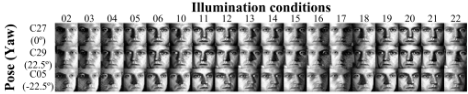
Data: We selected faces from the PIE database [Sim et al., 2003] to form paired tensor sets of different poses. Three poses C27, C29 and C05 were selected, corresponding to Yaw angle of 0, 22.5 and -22.5 degrees, as shown in Fig. 2. This subset includes faces from 68 subjects captured under 18 illumination conditions (02 to 06 and 10 to 22), where 07 to 09 were excluded due to missing faces. Thus, we have 68 × 3 × 18 = 3, 672 faces for this study. All face images were cropped, aligned with annotated eye coordinates, and normalized to 32 × 32 pixels with 8-bit depth.

Algorithm settings: We denote MCCA with Architectures I and II as MCCA1 and MCCA2, respectively. We also examine their fusion to see whether they contain complementary information using score level fusion with a simple sum rule, denoted as MCCA1+2. They are compared against CCA 3 and 2D-CCA [Lee and Choi, 2007]. We set the maximum number of iterations to ten for 2D-CCA and MCCA. We initialize the projection matrices in 2D-CCA to identity matrices, which gives better performance than random initialization in our study. We extract the maximum number of features for each method (32 for MCCA, 1024 for 2D-CCA and CCA). The extracted features are sorted according to the correlations captured in descending order. Face images are input directly as 32 × 32 matrices to 2D-CCA and MCCA. For CCA, they are reshaped to 1024 × 1 vectors as input.

Convergence study: Figure 3(a) depicts an example of the correlations captured over up to 20 iterations during learning for the first five canonical variates of MCCA1. Typically, the correlation captured improves quickly in the first a few iterations and tends to converge over iterations.

Feature correlations: Next, we examine whether the studied methods produce same-set and cross-set uncorrelated features. Figures 3(b) and 3(c) plot the average correlations of the first 20 features with all the other features in the same set and in the other set, respectively, excluding correlations between the same pairs. Correlations are nonzero in both cases for 2D-CCA. In contrast, CCA features are uncorrelated in both cases, while MCCA1 and MCCA2 have achieved sameset and cross-set zero-correlations, respectively, as supported by derivation in Sec. 3.2. Furthermore, the same-set correlations for MCCA2 and the cross-set correlations for MCCA1 are both low, especially for the first few features. This indicates that they may have similar performance.

Learning and matching: Finally, we investigate how well

3 Code by D. Hardoon: http://www.davidroihardoon.com/

Professional/Code files/cca.m MCCA can learn a mapping between face images of different poses. We divide the PIE subset into training set and test set and perform 10-fold cross validation with respect to subjects. Thus, the training set contains Pose1-Pose2 pairs of 61/62 subjects and the test set contains Pose1-Pose2 pairs of the rest 7/6 subjects (no overlapping). We study three pose pairings: C27-C29, C27-C05, and C29-C05. Figure 3(d) shows the design of this experiment.

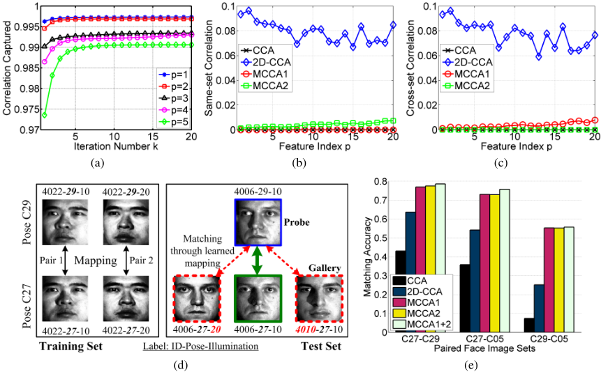
For each Pose1-Pose2 pairing, we evaluate the matching performance on the test set after training. The gallery consists of G(= 108/126) images of Pose1, projected to {rg}, g = 1, ...,G, through learned Pose1 subspace. The probe consists of the same number of Pose2 images. Each probe image is projected to a vector s in learned Pose2 subspace. With learned canonical correlations {ρp}, we predict the mapping of s to Pose1 as ˆr ∈ RP , where its pth element is ˆ rp = ρpsp [Weenink, 2003]. The best match is then ˆ g = argming dist(ˆr, rg), where dist(·) is a distance measure. We test three measures to find the best results: L1 distance, L2 distance, and angle between feature vectors [Lu et al., 2008]. A correct match is found when the probe and gallery images differ only in pose. The matching is incorrect even if the probe and gallery images are of the same subject but of different illuminations, as illustrated in Fig. 3(d). We report the best results from testing up to 32 features for MCCA and up to 1024 features for CCA and 2D-CCA.

Figure 3(e) depicts the matching results on three pose pairings. Despite having much fewer features (only 32 1024 = 1 32 ), MCCA-based methods give the best matching performance for all three scenarios, showing the effectiveness of uncorrelated features and direct learning of compact representations from tensors. There is a small improvement by fusing MCCA1 and MCCA2, implying that they are slightly complementary.

5 Conclusions

We proposed a multilinear CCA method to extract uncorrelated features directly from tensors via tensor-to-vector projection for paired tensor sets. The algorithm successively maximizes correlation captured by each projection pair while enforcing the zero-correlation constraint under two architectures. One architecture produces same-set uncorrelated features while the other produces cross-set uncorrelated features (except the paired features). The solution is iterative and alternates between modes. We evaluated MCCA on learning the mapping between faces of different poses. The results show that it outperforms CCA and 2D-CCA using much fewer features under both architectures. In addition, the two architectures complement each other slightly.

Acknowledgments

The author would like to thank the anonymous reviewers of this work for their very helpful comments.