Online Hashing

1 Introduction

Finding nearest neighbors using machine learning algorithms has achieved a widespread success in many applications, e.g. computer vision and text retrieval problems. However, due to the dramatic increase in the scale and dimension of data in the real world, those frequently using nearest neighbor search algorithms that exhaustively scan the dataset have become impractical for processing large-scale data in the real-world applications. To solve this problem, hashing-based searching methods have been developed to allow searching into a collection of millions of samples in a constant time.

Early works construct hash functions based on random projection, among which Locality-Sensitive Hashing (LSH) [Charikar, 2002] and its variants including ℓp-stable hashing [Datar et al., 2004] and min-hash [Chum et al., 2008] are the most representative methods. Though these methods obtains high accuracy, they are data-independent and need long codes to guarantee the performance.

In contrast to data-independent hashing methods, recently a great number of researches pay much attention to datadependent hashing learning algorithms, which can utilise label information of data, their distribution information and similarity between data as well. The objective of these methods is to obtain compact codes fitting data distribution in the feature space. Data-dependent hashing methods are usually grouped into three categories: unsupervised (for example [Weiss et al., 2008; Salakhutdinov et al., 2007]), semisupervised (such as [Wang et al., 2010]), and supervised methods (for instance [Liu et al., 2012]). The last two categories take advantage of label information [Wang et al., 2010] or pair-wise information [Mu et al., 2010] of points. These methods aim to minimise a cost function on the hash function set, formulated by combining an error term (to fit training data) and a regularisation term (to avoid over-fitting).

Although data-dependent hashing methods require fewer hash codes to obtain good performance than data-independent methods, they are all batch mode learning methods and have to involve a gigantic training labelled data set to obtain a good model. Also, existing learning based hashing methods assume all training data are available in advance for training and learn hash functions once for all. However, training on large scale data would result in a great deal of computational time and memory, which the real-world application cannot stand. Furthermore, in the real world application, it could be necessary to make hashing model adapted to new data.

In this paper, we overcome the limitation of batch mode methods by developing an online hashing learning method. For learning hash functions in an online manner, we develop a kernel mapping based passive-aggressive learning strategy for accommodating a new pair of data. The hashing model aims to construct hash functions to map the data points to finite number of hash codes, meanwhile appropriately preserving the distances or semantic relationship between data. By utilising passive-aggressive strategy [Crammer et al., 2006], the newly learned hashing model is able to retain important information learned in the previous rounds and optimise for data of current round as well. We can further derive bounds on the cumulative loss of the proposed online algorithm, guaranteeing better performance of online learning.

As far as we know, the proposed online learning specially designed for hash function learning in this work might be the first attempt. Although the minimal loss hashing(MLH) [Norouzi and Fleet, 2011] is an iterative algorithm and might be extended for learning new data, MLH is designed to minimise the max loss function for all pairs of samples over the whole training set rather than to update hash functions on each pair of data received step by step. Besides, it is not specially designed to learn hash function online, and thus the performance of MLH is not theoretically guaranteed for online learning.

2 Online Modelling

2.1 Preliminary

Hashing algorithms map a given data point z ∈ Rd into an r-bit binary code h ∈ {-1, 1}r . To deal with linearly inseparable data, kernel trick is used to tackle the data to improve the performance. Such a process has been theoretically and empirically shown to be an effectual approach for hash function learning [Kulis and Grauman, 2009; Liu et al., 2012]. In this paper, our online learning is built in this line. We first introduce the kernel mapping φ. For modeling this mapping, we follow [Liu et al., 2012] to preprocess original input data by mapping a d-dim vector z to a m-dim kernel vector φ(z) with the kernel function κ as

where z(1), z(2), ..., z(m) are m samples uniformly selected at random from data available. Since samples available at the preprocessing stage may be less than m because our algorithm is for online learning, we would use the first m samples received to construct φ, and our algorithm will start after m samples have been received.

For convenience of notation, we define x = φ(z). For r-bit linear projection hashing, the kth hash function is defined as

where wk ∈ Rm is a projection vector, bk is a threshold, and hk ∈ {-1, 1}. For r bit hash codes, we can redefine wk to be [wk T , bk]T and redefine x to be [xT , 1]T , and therefore our hash function becomes

where W = [w1,w2, ...,wr] ∈ R(m+1)×r is the hash projection matrix and h = [h1(x), h2(x), ..., hr(x)]T . The hash projection matrix W is learned by some criterion.

More specifically, the sign function in Eq. (1) is nondifferentiable, making it hard to model the optimization problem. Inspired by the structured prediction in structured SVMs [Finley and Joachims, 2008] and Minimal loss hashing [Norouzi and Fleet, 2011], we re-express the hash function equivalently as a form of structured prediction:

2.2 Online Learning Algorithm

Our proposed online hashing learning algorithm, which we call the Online kernel-based Hashing(OKH), is to process hashing model update for each new available pair of data point xti and xtj in tth , (t = 1, 2, ...) round. We denote such a pair by t = [xti , xtj ]. In addition, we assume that it is able to know whether these two points are similar or not by a similarity label. The similarity label s is given as follows:

Given the hash projection matrix Wt learned in the last round, we can derive the hash codes for xti and xtj denoted by hti , htj , respectively. We let t = [hti , htj ] denote the pair of hash codes. However, the generated hash codes usingWt could not be discriminant, as they may differ too much for two similar points or in contrast keep too similar for two dissimilar points. Hence, an optimal Wt+1 has to be learned.

In order to learn the new hash projection matrix, our idea is to use the labelled information which tells the pair is similar or not to derive an optimal hash codes t = [gt i , gt j ]. And then, we utilise this new hash codes t to guide the learning of new hash projection matrix Wt+1 , which can be viewed as a regression like process.

First, we introduce the loss of hash codes w.r.t. the similarity score s as follows

where fi and fj are hash codes of date pair obtained by W, = [fi, fj], Dh(fi, fj) is the Hamming distance between fi and fj, and α is a Hamming similarity threshold ranging from 0 to 1. The loss function above is to tell that the Hamming distance between similar points should be smaller than (1 - α)r, while the distance between non-similar points should be larger than αr. If not, we should penalise hash function learning to approach minimizing ℓ( , s).

We claim that we can compute an optimal hash code t for t such that ℓ( t , st ) = 0. We leave it to detail in Sec. 3. Now, we focus on computing an updatedWt+1 upon the optimal t . Let us define

Given hash function Eq.(2) with Wt , since hti and htj are the solution for xti and xtj , respectively, we have Ht (Wt ) ≥ Gt (Wt ). Define ̂t is the hash codes of t computed using updated Wt+1 by Eq. (2). Now we aim to get an Wt+1 to ensure ̂t approximate to t . Therefore, Wt+1 should meet the condition that Gt (Wt+1 ) > Ht (Wt+1 ). To achieve this objective, we derive the following prediction-based loss function ℓPB(W; t , t , st ) for our algorithm following the prediction-loss function in [Crammer et al., 2006],

Here we utilise the square root of loss function ℓ, because it can provide us a tighter bound on cumulative loss (Sec.2.4) Note that if ℓPB(Wt+1 ; t , t , st ) = 0, we can have Gt (Wt+1 ) =Ht (Wt+1 )+√ℓ( t , st ) >Ht (Wt+1 ). Even though this cannot guarantee that ̂t is exactly t , it is probable that ̂t is very close to t rather than t . It therefore makes sense to force ℓPB to be zero or close to zero.

Besides, in order to preserve the information learned in the last round, we constrain that the new learnedW should stay as close toWt as possible. Hence our objective function for updating hash projection matrix becomes

where ξ is a non-negative auxiliary variable in order to minimise prediction-based loss function ℓPB(W; t , t , st ), C is a positive parameter named aggressiveness parameter. It controls the effect of slack term and therefore controls the margin of update. Besides, is considered as a constant rather than dependent variable of W.

The proposed online hashing model above is in sense of a passive-aggressive strategy [Crammer et al., 2006]. The passive in our online hashing learning means Wt+1 = Wt whenever the loss is zero, and it is aggressive when the loss is positive and then the model will learnWt+1 to satisfy the constraint ℓ( ̂t , st ) = 0 as much as possible and meanwhile makeWt+1 not differ fromWt too much.

2.3 Optimization

The optimization is summarised in Algorithm 1. We now give the details. For convenience, we denote ℓPB(Wt ; t , t , st ) by ℓtPB . We focus on the solution when ℓt > 0. We first formulate the Lagrangian of the optimization problem Eq. (5) as follows

where τ t ≥ 0 and λ ≥ 0 are Lagrange multipliers.

We know that the optimal solution is the one satisfying ∂L/∂W = 0, ∂L/∂ξ = 0, and ∂L/∂τ t = 0.

Based on the above conditions, we can deduce the following formulations:

By putting Eqs. (7) and (8) back into Eq. (6), we get

Taking the derivative of L with respect to τ t and setting it to zero leads to:

Since τ t < C, we obtain

Thus, the solution of the optimisation problem in Eq. (5) is

Algorithm 1 Online Kernel-based Hashing

INITIALIZE W1

for t = 1,2,... do Receive pairwise instances: t Map t into kernel vector t Compute hash code t for t by Eq. (1) or Eq. (2) Receive similarity label st Compute loss by Eq. (3) if ℓ ̸= 0 then Get t for solution to ℓ( t , st ) = 0 Compute prediction-based loss ℓtPB by Eq. (4) Set τ t = min{C, ℓtP B || t( tt)T ||2 } Update Wt+1 = Wt + τ t t ( t - t )T elseWt+1 = Wt end if end for

2.4 Loss Bound

Following the analysis in [Crammer et al., 2006], we state similar relative bounds for our online hashing learning algorithm. For convenience, at the step t we define

where U is an arbitrary matrix in R(m+1)×r .

Based on the Lemma 1 and Theorem 2 in [Crammer et al., 2006], we can obtain the following lemma and theorem.

Lemma 1 Let ( 1 , s1 ), · · · , ( t , st ) be a sequence of pairwise examples with similarity label st ∈ {-1, 1} for all t. The data pair t ∈ R(m+1)×2 are mapped to a r-bit hash pairwise code t ∈ Rr×2 . Let U be an arbitrary matrix in R(m+1)×r . If τ t is defined as in Eq. (11), then

whereW1 is initialised to be nonzero matrix.

Theorem 2 Let ( 1 , s1 ), · · · , ( t , st ) be a sequence of pairwise examples with similarity label st ∈ {-1, 1} for all t. The data pair t ∈ R(m+1)×2 are mapped to a r-bit hash pairwise code t ∈ Rr×2 and || t ( t - )T ||2 is bounded by F 2 . Then for any matrix U ∈ R(m+1)×r , the cumulative loss suffered on the sequence is bounded, i.e.

where C is the aggressiveness parameter.

Note that it is possible that there exists a matrix U satisfying ℓtU = 0 for all t. Therefore, the cumulative loss is bounded by F 2 ||U - W1 ||2 . Due to limit of the length of the paper, we omit the proof of the above lemma and theorem. As ℓ( t , st ) is bounded, it guarantees the performance of the hash model for unseen data.

3 Optimal Hash Code Inference

In Sec.2.2, our online hashing algorithm relies on t = [gi t , gj t ] which satisfies ℓ( t , st ) = 0. Now, we detail how to acquire this kind of t . Due to the length of paper, we only discuss the case of dissimilar pairs and the processing for similar pairs can be similarly developed.

As mentioned in Sec.2.1, to achieve zero loss, the Hamming distance between the hash codes of non-neighbors should be larger than αr. Therefore, we only need to seek t such that Dh(gi t , gj t ) ≥ αr. Denote the kth bit of hi t as hi t[k] , and similarly for hj t , gi t , gj t . Therefore, Dh(hi t , hj t ) = ∑rk=1 Dh(hi t[k] , hj t[k] ), where

Let K1 = {k|Dh(hi t[k] , hj t[k] ) = 1} and K0 = {k|Dh(hi t[k] , hj t[k] ) = 0}. To obtain t , we set gi t[k] = hi t[k] and gj t[k] = hj t[k] for k ∈ K1. This is to retain the Hamming distance which tells non-similarity using the hash functions in previous round. For k ∈ K0, where hi t[k] = hj t[k] , we only need to set either gi t[k] = -hi t[k] or gj t[k] = -hj t[k] , so that we can have Dh(gi t[k] , gj t[k] ) = 1. Thus we can pick up p bits whose indexes are in set K0 such that

We next show it is not necessary to update all the rest hash bits w.r.t. K0. Note that W consists of r projection vectors wk(k = 1, 2, ..., r). From Eq.(7), we can deduce that

It can be found that wt+1 k = wtk , when gi t[k] = hi t[k] and gj t[k] = hj t[k] . Otherwise wtk will be updated. Note that if we update most wk inW, then we subsequently have to update all the corresponding hash bits of all data points.This does take severely much time and cannot be ignored for online applications. Hence, we aim at changing hash bits as few as possible; in other words, we aim to update wk as few as possible (i.e. p is as small as possible) and meanwhile ensure finding t such that ℓ( t , st ) = 0.

Following the above discussion, the minimum of p is p0 = αr - Dh(hi t , hj t ) by setting Dh(gi t , gj t ) = αr, because p = Dh(gi t , gj t ) - Dh(hi t , hj t ) and Dh(gi t , gj t ) ≥ αr. This can be done by selecting the p0 hash bits whose indexes are in K0. Since Ht (Wt ) predicts the error hash codes in Eq. (2), the bits contributing most for this mistaken Ht (Wt ) should be selected to update. We define the contribution of every bit w.r.t Ht by

We only select the largest one between hi t[k]wtk T xi t and hj t[k]wtk T xj t because we will never set t simultaneously by gi t[k] ̸= hi t[k] and gj t[k] ̸= hj t[k] for any k ∈ K0. Then the p0

Algorithm 2 Inference of t for Dissimilar Pair

1. Calculate the Hamming distance between hi t and hj t
2. Calculate p0 = αr - Dh(hi t , hj t )
3. Compute δk for k ∈ K0 by Eq. (14)
4. Sort δk
5. Set the corresponding hash bits of the p0 largest δk to be different from t and the others to be the same as t

largest δk are picked up and their corresponding hash bits are selected for update.

Nowwe summarise the procedure of obtaining t in Algorithm 2 Finally, a serious matter is that the rule for selecting the top p0 hash bits above won't work if wtk is a zero vector, because δk = 0 no matter what values hi t[k] , hj t[k] , xi t and xj t are. To avoid this situation, we initialise W1 to be an unfolded identity matrix WE which has 1's on the diagonal and zeros elsewhere. To accelerate the update progress, we initialise W1 using LSH denoted as WLSH, i.e. W1 are sampled from a zero-mean multivariate Gaussian N (0, I).

4 Experiments

To evaluate algorithms' performance in semantically similar neighbors searching and metric distance neighbors searching, we run large-scale image retrieval experiments on two datasets: Photo Tourism [Snavely et al., 2006] and 22K LabelMe [Torralba et al., 2008].

4.1 Dataset

Photo Tourism consists of photo collections in 3D with 3 subsets, and each contains about 100K patches of resolution 64×64 grayscale. Each set contains the match information indicates where it comes. We selected one of the subsets which consists of 104K patches taken from Photo Tourism reconstructions from Half Dome in Yosemite. In the experiment, we use 512-D Gist Features to describe each patch and partition the dataset into two parts: a training set consists of 98K pathes and a testing set consists of 6K patches. The pairwise labels s are obtained from the match information.

22K LabelMe contains 22,019 images. In our experiment, each image is represented by a 512-D Gist descriptor as well. Additionally, we just randomly selected 2K images from the dataset as test set, and set the remaining images as training set. Since label information is unavailable, neighbors are defined by the threshold in the Euclidean Gist space. The rule is: the label of a query and another point is set to s = 1 (i.e. they are similar) if the their Euclidean distance is within top 5% of the whole 20K distance and otherwise s = -1 (i.e. they are not similar). In our experiments, each training point has 110 neighbors.

4.2 Comparison

We compare the proposed algorithm with related methods in the following 2 aspects: 1) Mean Average Precision (MAP) [Turpin and Scholer, 2006; Wu et al., 2012] using Hamming ranking; 2) training time.

Since, as far as we know, it could be the first attempt to develop online kernel hashing learning model for learning sequential pair of data points, we selected two related batch mode hashing methods for comparison: 1) KLSH [Kulis and Grauman, 2009] and 2) minimal loss hashing(MLH) [Norouzi and Fleet, 2011]. KLSH is a variant of LSH [Charikar, 2002] using kernellised projection vectors in place of random projection vectors. MLH deals with similar hash function (Eq. (2)) as in our algorithm and aims at minimising the cumulative loss for all the pairwise samples in the whole training set. Although both MLH and OKH are supervised hashing methods, MLH is batch mode hashing learning over the whole training set, while our method is online based method which does not assume all training data are available in advance and learns just based on the data of current round. In our experiment, we feed OKH and KLSH the Gaussian RBF kernel κ(x, y) = exp(-||x - y||2 /2σ2 ) and m = 300 support samples on each dataset. The kernel parameter σ is fixed to be data variance, namely 1.3 for Photo Tourism and 0.8 for LabelMe. As MLH is not a kernel based method, it thus performs directly on input data.

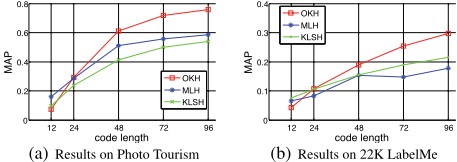
Regarding the use of training data, only MLH and our OKH are learning based methods. MLH is batch-based and hence all the training data will be used for learning the model. Since OKH processes the learning upon on a pair of data points in each round, we uniformly selected two samples from the training set at randomwithout replacement. For experiments on Photo Tourism, OKH has 49K pairs input and MLH utilises the same 98K samples for training; on 22K LabelMe, OKH has 5K pairs of samples and MLH utilises the same 10K data points. Because OKH learns a new model at every step. Hence its performance is set to be the average value of the MAP of the models learned at the step from t > 1000 to the end.

Fig. 1 shows the results of MAP comparison. Clearly, we can see that our algorithm outperforms the other two methods with clear margin when the hash code length increases. On Photo Tourism, the largest gain in MAP of OKH is nearly 30% more over MLH and 40% more over KLSH at 96 bits; on 22K LabelMe, the OKH gains 60% higher accuracy than MLH at 72 bits, and more than 30% higher than KLSH at 96 bits. This suggests: 1) OKH learns the hashing model from nothing and gains a clear better model than KLSH which is random model; 2) although only learn/update hashing model based on a pair of data in each round, OKH is able to get an more excellent performance than some batch mode hashing models; 3) benefited from online learning, OKH can process kernelised feature vectors efficiently, while it could be challenging for MLH, although kernel version of MLH can be derived beyond [Norouzi and Fleet, 2011].

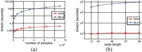
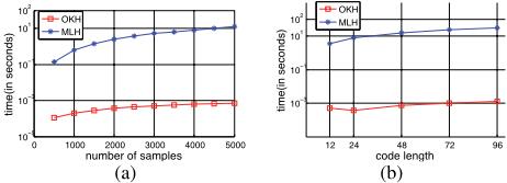
Regarding training time comparison, Fig. 2 and Fig. 3 shows the comparison results for different methods. It is clear that our algorithm takes much less time. This validates that our algorithm is a real-time algorithm and can be applied to the real-world large scale problem.

Moreover, from Fig. 2(b) and Fig. 3(b), we can clearly see that the time OKH takes to train hashing model increases very little with the hash code length growing. On the other hand, in Fig. 2(b), when it comes to 48 bits, the time does not increase when the further increasing hash bit length. Perhaps, this is because with more hash bits, our algorithm can learn better hash functions which will not cause any loss at most steps, resulting that the overall training time does not increase.

4.3 Parameter affect

We now evaluate effect of the parameters of OKH.

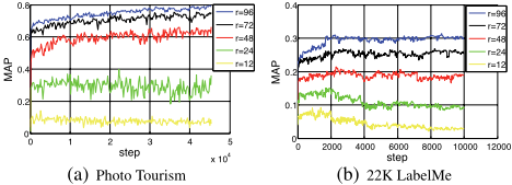
Code Length r. First, we report the performance of our method as a function of the hash code length r, where we fix α = 0.3 and C = 0.01 on Photo Tourism and α = 0.2 and C = 0.1 on 22K LabelMe . In addition, we initialise W1 as WLSH, which is the hashing model used by KLSH.

In Fig. 4, OKH performs better as the number of bits increase. Especially, when the hash bit length is less than 48, the performance is dramatically better and better as r becomes larger. However, when r is larger than 48, the improvement becomes less as r increases. Whereas as we know, the storage of hash codes increases linearly w.r.t. the growth of r. Therefore, an appropriate code length (e.g. r = 48) should be considered in order to balance the storage and accuracy.

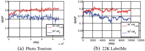
Initialisation of W. In Sec.2.4, we state that the initialisation of W may have a great influence on our algorithm because the bound of the cumulative loss is related to it. To address this concern, we evaluate the effect of different initiations of W here. Similar to the previous experiments, we set the length of hash bits to 48 and fix the other parameters the same as the setting in the last section on two datasets. As mentioned in the preceding part, in our experiment, we initialise W through two tricks: an unfolded identity matrix WE with 1s on the diagonal and 0s elsewhere and a matrix WLSH sampled from a zero-mean multivariate Gaussian N(0, I). Fig. 5 presents the results of different W1 . It is clear that our algorithm initialised withWLSH achieves better performance than the one withWE, which means that the initialisation plays an important role in our algorithm. In addition, using initialisationWE, our algorithm fluctuates more fiercely than usingWLSH as shown in Fig. 5. This is because the initialisation usingWLSH enjoys a lower cumulative loss bound by Theorem 2 and therefore it is easy to get to a stable status while the W1 = WE makes our method stay long in the oscillating status. Moreover, it is convenient and easy to get WLSH. Hence, we set WLSH as a default initialisation. Similarity Threshold α. In order to observe the effect of similarity threshold α on our algorithm, we vary α from 0.1 to 0.8. and fix the other parameters byW1 = WLSH, r = 48 and C is the same as the previous two experiments. As described in Eq.(3), we can regard α as similarity threshold because it tells whether a pair of points is similar or dissimilar in the Hamming space. Fig. 6 depicts how the parameter α affects the performance of the algorithm. The results indicate that α is an significant part in our algorithm. A small α (e.g.α = 0.1 in this experiment) allows the model to update smoothly. However, it also allows no update for much more hash code pairs with neutral Hamming distance between αr and (1 - α)r, regardless of its similarity s. This would lead to ordinary performance of the hashing model. On the other hand, a large α could make it hard for many data pairs to fit the loss function, and therefore it may cause fluctuating performance. This can be experimentally verified by Fig. 6(a)

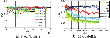
when α > 0.3. As a result, we would like to suggest an appropriate α ranging from 0.2 to 0.3.

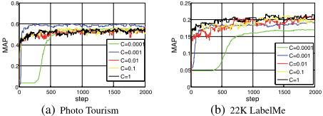
Aggressiveness Parameter C. We evaluate the performance of OKH on the first 2000 rounds with different C ranging from 0.0001 to 1. In this experiment, α is set to be 0.3 for Photo Tourism and 0.2 for 22K LabelMe. For the other parameters, they are set the same as the ones used in the previous experiments. Fig. 7 shows that the aggressiveness parameter C affects the convergence speed of our algorithm and the vibration as well. A small C causes slow improvement, e.g. C = 0.0001. In contrast, a much larger C results in fluctuation. If between, e.g. C = 0.001 in Fig.7(a), it achieves a higher performance than any other. In Fig.7(b), its MAP is generally a little lower than those of larger C, but its MAP fluctuates within a narrow range. Consequently, the aggressiveness parameter should be neither too small nor too large.

5 Conclusion

We propose an online hashing learning method called online kernel-based hashing, which updates a hashing model in each round based on a pair of data. Our online learning guarantees that the updated hashing model is optimal for current pair of data and gains a tight bound for new arriving pair. Empirical results on different datasets show that our approach gains satisfactory results, although it does not assume all training data are available in advance. It is promising that our proposed online hashing model can be a useful tool to address real-world problems with gigantic data set for online searching.

6 Acknowledgements

This research was supported by the National Natural Science of Foundation of China (No.61102111), the NSFC-GuangDong (U1135001), Foundation of China and Royal Society of Edinburgh (NSFCRSE) joint project (No.61211130123), Specialized Research Fund for the Doctoral Program of Higher Education (No.20110171120051), Guangdong Natural Science Foundation (No.S2012010009926), the Fundamental Research Funds for the Central Universities (No.12lgpy28, 2012350003161455) and the Guangdong Provincial Government of China through the Computational Science Innovative Research Team program.