
Efficient Kernel Learning from Side Information Using ADMM
Proceedings of the Twenty-Third International Joint Conference on Artificial Intelligence. Pages 1408-1413.
© 2013 International Joint Conferences on Artificial Intelligence
Abstract
Side information is highly useful in the learning of a nonparametric kernel matrix. However, this often leads to an expensive semidefinite program (SDP). In recent years, a umber of dedicated solvers have been proposed. Though much better than off-the-shelf SDP solvers, they still cannot scale to large data sets. In this paper, we propose a novel solver based on the alternating direction method of multipliers (ADMM). The key idea is to use a low-rank decomposition of the kernel matrix K = VT U, with the constraint that V = U. The resultant optimization problem, though non-convex, has favorable convergence properties and can be efficiently solved without requiring eigen-decomposition in each iteration. Experimental results on a number of real-world data sets demonstrate that the proposed method is as accurate as directly solving the SDP, but can be one to two orders of magnitude faster.
- [Bach et al., 2004] F.R. Bach, G.R.G. Lanckriet, and M.I. Jordan. Multiple kernel learning, conic duality, and the SMO algorithm. In Proceedings of the Twenty-First Inter- national Conference on Machine, Banff, Alberta, Canada, July 2004.
- [Belkin et al., 2006] M. Belkin, P. Niyogi, and V. Sind- hwani. Manifold regularization: A geometric framework for learning from labeled and unlabeled examples. Journal of Machine Learning Research, 7:2399-2434, 2006.
- [Boyd et al., 2011] S. Boyd, N. Parikh, E. Chu, B. Peleato, and J. Eckstein. Distributed optimization and statistical learning via the alternating direction method of multipli- ers. Foundations and Trends in Machine Learning, pages 1-122, 2011.
- [Burer and Choi, 2006] S. Burer and C. Choi. Computa- tional enhancements in low-rank semidefinite program- ming. Optimization Methods and Software, 21(3):493- 512, 2006.
- [Chapelle et al., 2003] O. Chapelle, J. Weston, and B. Schölkopf. Cluster kernels for semi-supervised learning. In Advances in Neural Information Processing Systems, 2003.
- [Cortes et al., 2009] C. Cortes, M. Mohri, and A. Ros- tamizadeh. Learning non-linear combinations of kernels. In Advances in Neural Information Processing Systems, 2009.
- [Fine and Scheinberg, 2001] S. Fine and K. Scheinberg. Ef- ficient SVM training using low-rank kernel representa- tions. Journal of Machine Learning Research, 2:243-264, December 2001.
- [Glowinski and Marrocco, 1975] R. Glowinski and A. Mar- rocco. Sur l'approximation, par elements finis d'ordre un, et la resolution, par penalisation-dualite, d'une classe de problems de dirichlet non lineares. Revue Francaise d'Automatique, Informatique, et Recherche Opérationelle, 9:41-76, 1975.
- [Golub and Van Loan, 1996] G.H. Golub and C.F. Van Loan. Matrix Computations. Hopkins University Press, Balti- more, Maryland, USA, 3rd edition, 1996.
- [Hoi et al., 2007] S.C.H. Hoi, R. Jin, and M.R. Lyu. Learn- ing nonparametric kernel matrices from pairwise con- straints. In Proceedings of the Twenty-Fourth International Conference on Machine Learning, pages 361-368, Corval- lis, Oregon, USA, June 2007.
- [Hu et al., 2011] E.-L. Hu, B. Wang, and S. Chen. BCD- NPKL: Scalable non-parametric kernel learning using block coordinate descent. In Proceedings of the Twenty- Eighth International Conference on Machine Learning, pages 209-216, Bellevue, WA, USA, June 2011.
- [Kulis et al., 2009] B. Kulis, M. Sustik, and I. Dhillon. Low-rank kernel learning with Bregman matrix diver- gences. Journal of Machine Learning Research, 10:341- 376, 2009.
- [Lanckriet et al., 2004] G.R.G. Lanckriet, N. Cristianini, P. Bartlett, L. El Ghaoui, and M.I. Jordan. Learning the kernel matrix with semidefinite programming. Journal of Machine Learning Research, 5:27-72, 2004.
- [Laue, 2012] S. Laue. A hybrid algorithm for convex semidefinite optimization. In Proceedings of the Twenty- Nineth International Conference on Machine Learning, pages 1206-4608, Edinburgh, Scotland, June 2012.
- [Li and Liu, 2009] Z. Li and J. Liu. Constrained clustering by spectral regularization. In Proceedings of the IEEE In- ternational Conference on Computer Vision and Pattern Recognition, pages 421-428, Miami, Florida, USA, June 2009.
- [Li et al., 2008] Z. Li, J. Liu, and X. Tang. Pairwise con- straint propagation by semidefinite programming for semi- supervised classification. In Proceedings of the Twenty- Fifth International Conference on Machine Learning, pages 576-583, Helsinki, Finland, July 2008.
- [Luxburg, 2007] U. Luxburg. A tutorial on spectral cluster- ing. Statistics and Computing, 17(4):395-416, December 2007.
- [Schölkopf and Smola, 2002] B. Schölkopf and A.J. Smola. Learning with Kernels. MIT Press, Cambridge, MA, 2002.
- [Shang et al., 2012] F. Shang, L.C. Jiao, and F. Wang. Semi- supervised learning with mixed knowledge information. In Proceedings of the Eighteenth Conference on Knowl- edge Discovery and Data Mining, pages 732-740, Beijing, China, August 2012.
- [Sonnenburg et al., 2006] S. Sonnenburg, G. Rätsch, C. Schäfer, and B. Schölkopf. Large scale multiple kernel learning. Journal of Machine Learning Research, 7:1531-1565, July 2006.
- [Vandenberghe and Boyd, 1996] L. Vandenberghe and S. Boyd. Semidefinite programming. SIAM Review, 38(1):49-95, 1996.
- [Wagstaff et al., 2001] K. Wagstaff, C. Cardie, S. Rogers, and S. Schroedl. Constrained K-means clustering with background knowledge. In Proceedings of the Eighteenth International Conference on Machine Learning, pages 577-584, Williamstown, MA, USA, June 2001.
- [Wu et al., 2009] X.-M. Wu, A. M.-C. So, Z. Li, and S.-Y.R. Li. Fast graph Laplacian regularized kernel learning via semidefinite-quadratic-linear programming. In Advances in Neural Information Processing Systems, pages 1964- 1972, 2009.
- [Xu et al., 2011] Y. Xu, W. Yin, Z. Wen, and Y. Zhang. An alternating direction algorithm for matrix completion with nonnegative factors. Technical Report TR11-03, Depart- ment of Computational and Applied Mathematics, Rice University, 2011.
- [Zhuang et al., 2011] J. Zhuang, I.W. Tsang, and S.C.H. Hoi. A family of simple non-parametric kernel learning algo- rithms. Journal of Machine Learning Research, 12:1313- 1347, 2011.
References were extracted automatically from the PDF and may contain errors.
Full text extracted automatically from the PDF; figures, tables and equations may differ. The PDF is the version of record.
1 Introduction
Kernel methods have been highly successful in various aspects of machine learning, such as classification, regression, clustering, ranking, and dimensionality reduction [Sch¨olkopf and Smola, 2002]. Because of the central role of the kernel, it is important to identify an appropriate kernel function or matrix for the task at hand. Over the past decade, there have been a large body of literature on this kernel learning problem [Lanckriet et al., 2004; Bach et al., 2004; Cortes et al., 2009]. While a parametric form of the kernel [Chapelle et al., 2003] or a combination of multiple kernels [Sonnenburg et al., 2006] are often assumed, nonparametric kernel learning, which takes no such assumptions, is more flexible and has received significant interest in recent years [Li et al., 2008; Wu et al., 2009; Kulis et al., 2009; Hu et al., 2011; Zhuang et al., 2011; Shang et al., 2012].
To facilitate kernel learning, obviously one has to utilize information from the data. The most straightforward approach is to use class labels. However, obtaining label information may sometimes be expensive and time-consuming. In this paper, we focus on a weaker form of supervisory information, namely, the so-called must-link and cannot-link pairwise constraints [Wagstaff et al., 2001]. These pairwise constraints, or side information, define whether the two patterns involved should belong to the same class or not. Another useful source of information, which is commonly used in semi-supervised learning, is the data manifold [Belkin et al., 2006]. This encourages patterns that are locally nearby on the manifold to have similar predicted labels.
A notable nonparametric kernel learning approach that nicely integrates these two sources of information is the pairwise constraint propagation (PCP) algorithm [Li et al., 2008]. Let n be the number of patterns, andM, C be the sets of mustlink and cannot-link pairs, respectively. PCP is formulated as the following optimization problem
where K = [Kij] ∈ Rn×n is the kernel matrix to be learned (which has to be symmetric and positive semidefinite (psd), denoted K ⪰ 0), L is the graph Laplacian matrix of the data manifold, T = [Tij ] with
T =M∪C∪{(i, i)}ni=1 , and γ is a regularization parameter. In words, the tr(KL) term in (1) encourages K to be aligned with L and thus smooth on the manifold, while (Kij - Tij)2 encourages Kij to be close to 1 for two must-link patterns i, j, and 0 for cannot-link patterns. Note from (2) that all the patterns are also encouraged to be normalized in the kernel representation (i.e., Kii ≃ 1).
As in other nonparametric kernel learning algorithms, the optimization problem in (1) is a semidefinite program (SDP) [Vandenberghe and Boyd, 1996]. Though off-theshelf solvers such as CSDP can be used [Li et al., 2008], they are slow, particularly when n is large or the pairwise constraints are abundant. Recently, Laue [2012] proposed a more efficient hybrid solver that is based on gradually increasing the rank of the K solution. However, each time the rank is increased, it has to perform an approximate eigen-decomposition and nonlinear optimization. As will be demonstrated in Section 4.2, this can be inefficient on large kernel learning problems.
Recently, there have been a lot of interest in scaling up this SDP. In many machine learning problems, a prominent tool that often drastically reduces the computational effort is lowrank approximation [Fine and Scheinberg, 2001]. In the context of kernel learning, this involves replacing the n×n matrix K by V⊤V, where V ∈ Rr×n and r is the rank. The solver in [Burer and Choi, 2006] can then be used, though the line search and computation of the coefficients in each iteration can be expensive. Alternatively, one can optimize V columnby-column using coordinate descent [Hu et al., 2011]. The resultant algorithm is scalable, but the decoupling of variables as required in coordinate descent makes it unable to handle the (soft) constraints of Kii ≃ 1 in (2).
Another popular low-rank approximation option is to replace K by QUQ⊤, as in [Li and Liu, 2009; Wu et al., 2009] and the modified fixed point continuation (MFPC) algorithm [Shang et al., 2012]. Here, Q ∈ Rn×r is a fixed matrix with orthogonal columns (usually the trailing eigenvectors of the graph Laplacian matrix L), and U ∈ Rr×r is the psd matrix to be optimized. Typically, r ≪ n, and thus optimization of U is much more manageable. Moreover, Wu et al. [2009] showed that problem (1) belongs to a special class of SDP called quadratic semidefinite program (QSDP). By exploiting this structure, they reformulated (1) as a semidefinitequadratic-linear program (SQLP), which reduces the complexity from O(n9 ) for the standard QSDP formulation to O(n6.5 ). However, empirically, this still does not scale well. As reported in [Wu et al., 2009], kernel learning on a data set with 2000 instances and 100 pairwise constraints takes about 4000 seconds. Moreover, the fixed Q limits the ability of K to fit the data, leading to possibly deteriorated performance of the learned model.
Instead of solving problem (1) directly, Zhuang et al. [2011] noted that this, together with other similar machine learning problems, can be reformulated as optimizing the inner product of the matrix variable with another fixed matrix. By adding an additional constraint tr(KK) ≤ B, where B > 0 is a user-defined constant, this optimization problem has a closed-form solution of K. The resultant algorithm, called simple nonparametric kernel learning (SimpleNPKL), is significantly more efficient than existing algorithms. However, computing the closed-form K solution requires eigendecomposition at each iteration, which can be expensive on large kernel learning problems with a large number of instances or constraints. Moreover, its performance is sometimes sensitive to the setting of B.
In this paper, our key idea is to decompose the matrix K as V⊤U, where V,U ∈ Rr×n , together with the constraint that V = U. Obviously, this is essentially the same as the commonly-used low-rank approximation V⊤V discussed above [Burer and Choi, 2006; Hu et al., 2011; Li and Liu, 2009], but with the important difference that V and U are now decoupled. Together with the QSDP structure in (1), this allows simple and efficient optimization based on the alternating direction method of multipliers (ADMM) [Boyd et al., 2011], which has been popularly used in diverse fields such as machine learning, data mining and image processing. Experimental results show that the proposed method is as accurate as solving the SDP directly, but is significantly more efficient and scalable.
The rest of this paper is organized as follows. Section 2 first gives a brief introduction to ADMM. Section 3 then describes the proposed solver and its properties. Experimental results on a number of real-world data sets are presented in Section 4, and the last section gives some concluding remarks.
Notations: In the sequel, matrices and vectors are denoted in bold, with upper-case letters for matrices and lower-case for vectors. The transpose of a vector/matrix is denoted by the superscript ⊤, tr(A) denotes the trace of matrix A, A⊙B is the element-wise multiplication of matrices A and B (i.e., [A⊙B]ij = AijBij), and A· B = tr(A⊤B) is their inner product. Moreover, I is the identity matrix, and 0 (resp. 1) is the vector (or matrix) of all zeros (resp. ones).
2 Alternating DirectionMethod of Multipliers (ADMM)
ADMM is a simple but powerful algorithm first introduced in [Glowinski and Marrocco, 1975], and has recently been successfully used in diverse fields such as machine learning, data mining and image processing. The standard ADMM is for solving convex problems. Here, we consider the more general bi-convex problem in [Boyd et al., 2011]:
where F (·, ·) is bi-convex and G(·, ·) is bi-affine 1 . As in the method of multipliers, ADMM considers the augmented Lagrangian of (3): L(x, y,Λ) = F (x, y) + Λ⊤G(x, y) + ρ2 ‖G(x, y)‖2 , where Λ is the vector of Lagrangian multipliers, and ρ > 0 is a penalty parameter. At the kth iteration, the values of x, y and Λ (denoted xk , yk and Λk ) are updated as
Note that while the method of multipliers minimizes L (x, y, Λk ) w.r.t. x and y jointly, ADMM allows easier decomposition of the optimization problem by minimizing them in an alternating manner.
3 Kernel Learning by ADMM
In this section, we present a novel solver for problem (1) based on the ADMM. Section 3.1 shows that the update steps can be efficiently computed. A necessary condition for convergence is provided in Section 3.2, and Section 3.3 discusses the time complexity in each iteration.
As in [Wu et al., 2009; Hu et al., 2011; Li and Liu, 2009], we use a low-rank approximation on the kernel matrix K. In other words, K is approximated as
where V ∈ Rr×n and rank r < n. Problem (1) can then be rewritten as
1 In other words, for any fixed x, y, F(·, y) and F(x, ·) are convex; while G(·, y) and G(x, ·) are affine.
Recall that the graph Laplacian matrix L is symmetric [Luxburg, 2007], this can be further written as
where U ∈ Rr×n , and vi's (resp. ui's) are the columns of V (resp. U). Note that the objective is bi-convex, and the constraint function V - U is bi-affine.
3.1 ADMMUpdate Steps
Let Λ be the Lagrangian multiplier for the constraint V - U = 0. As in Section 2, the augmented Lagrangian of (5) is
and the update steps at the kth iteration of ADMM are
It can be easily shown that
where
Λki is the ith column of Λk , and Ti = {j | (i, j) ∈ T }.
On setting (9), (10) to zero, the solutions of (7) and (8) can be obtained as
for i = 1, · · · , n. Note from (11), (12) that Aki and Bki are always invertible.
To monitor convergence of the algorithm, we require the primal and dual residuals at iteration k + 1
Δprimal = ∥∥Vk+1 -Uk+1∥∥ , Δdual = ρ ∥∥Vk+1 -Vk ∥∥ (14) to be small [Boyd et al., 2011]. Moreover, to improve convergence, it is common to vary the penalty parameter ρ in each ADMM iteration. Specifically, following [Boyd et al., 2011], we update ρ as
The whole procedure is shown in Algorithm 1.
Algorithm 1 KLADMM: Kernel learning by ADMM.
- 1: Input: rank r, V0 = [v0 1 , . . . , v0n ],U0 = [u01 , . . . , u0n ], parameters ρ, ε and IterMax.
- 2: Output: K = Vk⊤Vk (or Uk⊤Uk ).
- 3: k ← 0;
- 4: repeat
- 5: for i = 1 to n do
- 7: end for
- 9: compute the primal and dual residuals in (14);
- 10: update ρ using (15);
- 11: k ← k +1;
- 12: until max(Δprimal,Δdual) < ε or k > IterMax;
3.2 Convergence
With the low-rank decomposition in (4), problem (5) is nonconvex in V and so we can only consider local convergence [Boyd et al., 2011]. As in [Xu et al., 2011], we show below a necessary condition for local convergence.
Lemma 1 Let {(Uk , Vk , Λk )} be a sequence generated by Algorithm 1. If the sequence {Λk } is bounded and satisfies
then Vk - Vk+1 → 0 and Uk - Uk+1 → 0.
Proof 1 First, observe that L(U,V,Λ) is bounded, which follows from the boundedness of Λ and
Moreover, L is strongly convex w.r.t. each coordinate variable of vi and ui. For any vi, it holds that
for any △vi, where L(vi, ·) denotes that all the variables in (7) except vi are fixed. Moreover, v⋆ i is a minimizer of L (vi, ·) if
Note that vk+1 i is a minimizer of L (vi, ·) at the kth iteration. Then, on combining (17) and (18), we have
Similarly, one can show that
Using (17) - (20) and Λk+1 - Λk = ρ(Vk+1 - Uk+1 ), we have
Taking summation of the above inequality from 1 to ∞, and recall that L is bounded, then
Since the second term on the left is bounded, it follows that ∞∑ k=1 (∥∥Vk - Vk+1∥∥2 + ∥∥Uk -Uk+1∥∥2) <∞, fromwhich we immediately have Vk -Vk+1 → 0 and Uk -Uk+1 → 0.
■Proposition 1 Let {(Uk , Vk )} be a sequence generated by Algorithm 1. Then any accumulation point of {(Uk , Vk )} satisfies the Karush-Kuhn-Tucker (KKT) condition for problem (5).
Proof 2 From (13), we have
Lemma 1 implies that the left- and right-hand sides of (21), (22), (23) all go to zero, i.e.,
and thus the KKT conditions for problem (5), namely,
are satisfied.
■
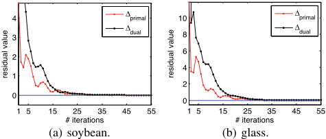
In particular, note from (24) that although the algorithm does not guarantee Uk = Vk at each iteration k, the difference goes to zero as the iteration proceeds. This will also be experimentally demonstrated in Section 4.1.
3.3 Time Complexity
As Aki ,Bki are of size r × r, computing their inverses in (13) takes O(r3 ) time. In practice, we often have r > Ti. For example, please refer to the experimental setup in Section 4. By rewriting Aki as γ ( ρ γ I + PiP⊤i ), where Pi = [ukj1 , . . . , ukj|Ti| ] ∈ Rr×|Ti| , and using the Sherman-MorrisonWoodbury (SMW) identity [Golub and Van Loan, 1996], we have
where ρ γ I + P⊤i Pi is of size |Ti| × |Ti|. Hence, computing (Aki )-1 takes only O(|Ti|3 + r|Ti|) time. The same applies to the computing of (Bki )-1 . The time complexity for each iteration of Algorithm 1 is then
In practice, |Ti| is usually very small, and (26) essentially scales linearly with n.
4 Experiments
As in [Hoi et al., 2007; Li et al., 2008], we study the performance of the proposed approach in the context of data clustering. Specifically, a kernel matrix is learned from the pairwise constraints, which is then used for clustering by the kernel k-means algorithm. Experiments are performed on a number of benchmark data sets (Table 1) that have been commonly used for nonparametric kernel learning [Hoi et al., 2007; Hu et al., 2011; Zhuang et al., 2011].
| data set | #classes | #patterns | #features | #constraints | avg(|Ti|) | r |
|---|---|---|---|---|---|---|
| chessboard | 2 | 100 | 2 | 340 | 2.2 | 25 |
| dbl-spiral | 2 | 100 | 3 | 340 | 2.2 | 25 |
| glass | 6 | 214 | 9 | 728 | 2.2 | 37 |
| heart | 2 | 270 | 13 | 918 | 2.2 | 42 |
| iris | 3 | 150 | 4 | 510 | 2.2 | 31 |
| protein | 6 | 116 | 20 | 396 | 2.2 | 27 |
| sonar | 2 | 208 | 60 | 708 | 2.2 | 37 |
| soybean | 4 | 47 | 35 | 161 | 2.2 | 17 |
| wine | 3 | 178 | 12 | 606 | 2.2 | 34 |
| adult-a1a | 2 | 1,605 | 123 | 5,457 | 2.2 | 103 |
| adult-a2a | 2 | 2,265 | 123 | 7,701 | 2.2 | 123 |
| adult-a3a | 2 | 3,185 | 123 | 10,829 | 2.2 | 146 |
| adult-a4a | 2 | 4,781 | 123 | 16,257 | 2.2 | 179 |
| adult-a5a | 2 | 6,414 | 123 | 21,808 | 2.2 | 208 |
| adult-a6a | 2 | 11,220 | 123 | 38,148 | 2.2 | 275 |
The constructions of the data manifold and pairwise constraints follow that in [Hoi et al., 2007; Hu et al., 2011;
Zhuang et al., 2011]. Specifically, the similarity between patterns xi, xj is defined as exp(-‖xi -xj‖2 /2σ2 ), where σ is equal to half of the average distance between each pattern and its top-10 nearest neighbor. The 50-nearest-neighbor graph is then used for the manifold of the adult data sets, and the 5nearest-neighbor graph for the others. As for the pairwise constraints, we randomly select 0.6n pairs of patterns that belong to the same class to construct the must-link pairs, another 0.6n pairs of patterns that belong to different classes to construct the cannot-link pairs, and another n must-link (i, i) pairs for each pattern i. On all the data sets, the average number of constraints (i.e., |Ti|) associated with a random pattern i is always around 2.
As for the rank of the kernel matrix, we follow [Zhuang et al., 2011; Hu et al., 2011] and set its value to be the largest r satisfying r(r + 1)/2 ≤ m, where m is the total number of constraints in T . Table 1 shows the rank values (i.e., r) used. As can be seen, they are all much larger than |Ti| ≃ 2, i.e., the average number of constraints associated with a random pattern i. This justifies the use of the SMW identity to compute the matrix inverse in Section 3.3.
The proposed KLADMM algorithm 2 is compared with the following solvers discussed in Section 1. Similar to KLADMM, all are based on a rank-r approximation of K.
- The hybrid algorithm [Laue, 2012], with the rank of the K solution increasing up to r;
- SimpleNPKL 3 [Zhuang et al., 2011], which is extended for the quadratic loss in (1);
- MFPC [Shang et al., 2012], which is based on the lowrank representation QUQ⊤, where the columns of Q are the r trailing eigenvectors of the graph Laplacian L;
- The SQLP solver [Wu et al., 2009], which is also based on the same low-rank representation as MFPC.
All the algorithms are implemented in MATLAB and run on a PC with i7-3370 3.4GHz CPU and 32G RAM.
The following performance evaluation measures are used:
- percentage of pattern pairs that are correctly clustered together [Hoi et al., 2007]:
where ci (resp. ˆ ci) is the true (resp. predicted) cluster label of pattern xi, and I (·) is the indicator function that returns 1 when the argument is true, and 0 otherwise;
- CPU time for learning the kernel matrix K.
4.1 Accuracy and Speed
Results on the clustering accuracy and CPU time are shown in Table 2. SQLP, which shares the same low-rank model as MFPC, has comparable accuracy as MFPC but is much slower (often by one to two orders of magnitude). Hence, its results are not reported here because of the lack of space. Moreover, some solvers become very slow on the larger data sets and so are not run to completion.
2V0 and U0 is initialized randomly, ρ = 100, and IterMax set to 500 (and to 100 on the adult datasets).
3 Recall that an additional B parameter is needed to constrain tr(KK). Preliminary results show that the solution quality can be sensitive to B. Here, we set B = 100n, which performs better in our experiments than the value suggested in [Zhuang et al., 2011].
As can be seen, KLADMM is much faster than SimpleNPKL, which in turn is faster than the hybrid algorithm. In particular, on the largest data set (adult-a4a) that SimpleNPKL can handle, KLADMM is about 30 times faster. MFPC, though is almost as fast as KLADMM, has much inferior accuracy, and cannot be improved even by increasing the size of U. As discussed in Section 1, for efficient optimization, MFPC has to fix the Q matrix in the low-rank representation (QUQ⊤) of K. This severely restricts the ability of K to adapt to the data.
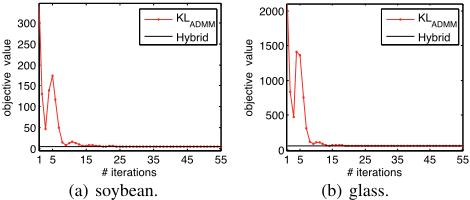
On the other hand, KLADMM, though involves non-convex optimization, is as accurate as the hybrid algorithm which converges to the globally optimal solution of the SDP problem [Laue, 2012]. Figure 1 shows the speed in which the objective value obtained by KLADMM converges towards the globally optimal objective of the hybrid algorithm. As can be seen, KLADMM often converges in fewer than 25 iterations.
Finally, Figure 2 shows the progress of KLADMM's primal and dual residuals with the number of iterations. Recall from (14) that the primal residual Δprimal measures the difference between Vk and Uk . As can be seen, this difference quickly goes to zero, as is discussed in Section 3.2.
| clustering accuracy | CPU time (sec) | |||||||
|---|---|---|---|---|---|---|---|---|
| data set | KLADMM | SimpleNPKL | (%) hybrid | MFPC | KLADMM | SimpleNPKL | hybrid | MFPC |
| chessboard | 91.28±4.17 | 89.09±5.33 | 91.28±4.22 | 71.09±4.87 | 3.08±0.05 | 17.06±0.34 | 38.95±3.57 | 1.22±0.23 |
| dbl-spiral | 99.70±0.96 | 98.71±1.27 | 99.70±0.96 | 99.68±2.31 | 0.74±0.23 | 10.44±0.40 | 15.61±2.62 | 1.32±0.06 |
| glass | 83.56±2.02 | 84.24±1.87 | 83.70±1.73 | 77.25±1.39 | 17.56±0.18 | 71.38±1.75 | 231.43±22.12 | 4.03±0.78 |
| heart | 78.88±2.79 | 78.03±3.93 | 79.00±2.75 | 58.34±4.09 | 37.14±0.16 | 113.85±2.73 | 400.60±37.63 | 5.64±0.45 |
| iris | 98.69±1.08 | 97.55±1.05 | 98.69±1.10 | 97.36±0.88 | 3.44±0.19 | 35.26±8.26 | 53.48±3.13 | 1.90±0.60 |
| protein | 90.34±2.21 | 87.93±1.97 | 90.27±2.20 | 85.39±1.87 | 3.91±0.18 | 22.44±0.56 | 54.34±4.23 | 1.66±0.17 |
| sonar | 91.54±2.49 | 89.53±2.34 | 91.59±2.54 | 71.84±3.39 | 16.28±0.21 | 62.35±2.20 | 174.27±15.22 | 3.39±0.13 |
| soybean | 98.73±3.84 | 96.10±5.07 | 98.73±4.40 | 93.80±5.85 | 0.77±0.18 | 1.96±0.09 | 5.80±0.73 | 0.20±0.11 |
| wine | 84.11±2.29 | 83.79±2.36 | 84.14±2.54 | 76.37±2.69 | 6.89±0.20 | 45.58±1.20 | 118.70±11.06 | 2.82±0.28 |
| adult-a1a | 95.85±1.35 | 85.68±2.06 | - | 66.29±1.83 | 54.99±0.78 | 365.68±26.33 | - | 120.42±14.32 |
| adult-a2a | 95.65±0.58 | 85.70±1.46 | - | 65.46±1.07 | 92.02±1.64 | 988.12±23.13 | - | 157.08±2.06 |
| adult-a3a | 93.16±0.93 | 83.68±1.07 | - | 62.07±2.31 | 161.60±3.25 | 2800.0±120.04 | - | 332.34±1.81 |
| adult-a4a | 93.23±0.46 | 82.97±0.62 | - | 61.94±2.82 | 319.29±2.71 | 8767.8±334.44 | - | 821.76±71.70 |
| adult-a5a | 92.93±0.44 | - | - | 63.21±0.88 | 1724.9±3.23 | - | - | 1407.0±135.92 |
| adult-a6a | 93.36±0.30 | - | - | 65.17±1.62 | 7661.7±4.20 | - | - | 4786.6±207.36 |
4.2 Scalability
In this section, we compare the scalability of the various algorithms, except for MFPC and SQLP which have been shown to have much inferior accuracy (Section 4.1). Experiments are performed on a synthetic 10-dimensional binary classification data set. Patterns from the first class are generated from the normal distribution N(1, I), while those from the second class are from N(-1, I).
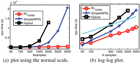
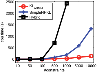
In the first experiment, we fix the number of constraints at 1,000. Figure 3(a) shows the CPU time as the number of patterns n increases. As in Section 4.1, KLADMM scales much better than the others. The curves are redrawn as a log-log plot in Figure 3(b). A line corresponding to a linear scaling between time and n is also shown. As can be seen, KLADMM scales almost linearly in n, which agrees with the analysis in Section 3.3. In the second experiment, we fix n at 1,000 and gradually increase the number of constraints (recall that the rank r also increases according to our experimental setup). Results are shown in Figure 4. As can be seen, KLADMM is again much more efficient than the other methods.
5 Conclusion
In this paper, we proposed an efficient solver for nonparametric low-rank kernel learning. Using ADMM, the proposed KLADMM decouples the original optimization problem into computationally inexpensive subproblems. Unlike existing solvers which perform a large eigen-decomposition in each iteration, KLADMM only requires operations on very small matrices. Experimental results on a number of real-world data sets demonstrate that KLADMM is as accurate as directly solving the SDP, but is much faster than existing solvers. Its CPU time scales linearly with the number of patterns, and can be used on much larger kernel learning problems.
In the future, the proposed solver will be extended to optimize other nonparametric kernel learning models.
Acknowledgment
This research was supported in part by the Research Grants Council of the Hong Kong Special Administrative Region (Grant No. 614012), the National Natural Science Foundation of China (No. 61165012) , the Natural Science Foundations Fund (Grant No. 2011FZ074) and the Department of Education Fund (No. 2011Y305) of Yunnan Province.
@inproceedings{ijcai2013p211,
  title     = {Efficient Kernel Learning from Side Information Using ADMM},
  author    = {Hu, En-Liang and Kwok, James T.},
  booktitle = {Proceedings of the Twenty-Third International Joint Conference on
               Artificial Intelligence, {IJCAI-13}},
  publisher = {AAAI Press / International Joint Conferences on Artificial Intelligence},
  editor    = {Francesca Rossi},
  pages     = {1408--1413},
  year      = {2013},
  month     = {8},
  url       = {https://ijcai.org/proceedings/2013/211},
}
TY - CPAPER TI - Efficient Kernel Learning from Side Information Using ADMM AU - Hu, En-Liang AU - Kwok, James T. T2 - Proceedings of the Twenty-Third International Joint Conference on Artificial Intelligence, IJCAI-13 PB - AAAI Press / International Joint Conferences on Artificial Intelligence PY - 2013 SP - 1408 EP - 1413 UR - https://ijcai.org/proceedings/2013/211 ER -Copied
Machine-readable versions of this paper, for tools and AI agents:





