
A Lossy Counting Based Approach for Learning on Streams of Graphs on a Budget
Proceedings of the Twenty-Third International Joint Conference on Artificial Intelligence. Pages 1294-1300.
© 2013 International Joint Conferences on Artificial Intelligence
Abstract
In many problem settings, for example on graph domains, online learning algorithms on streams of data need to respect strict time constraints dictated by the throughput on which the data arrive. When only a limited amount of memory (budget) is available, a learning algorithm will eventually need to discard some of the information used to represent the current solution, thus negatively affecting its classification performance. More importantly, the overhead due to budget management may significantly increase the computational burden of the learning algorithm. In this paper we present a novel approach inspired by the Passive Aggressive and the Lossy Counting algorithms. Our algorithm uses a fast procedure for deleting the less influential features. Moreover, it is able to estimate the weighted frequency of each feature and use it for prediction.
- [Alippi et al., 2012] Cesare Alippi, Manuel Roveri, and Francesco Trovò. A "learning from models" cognitive fault diagnosis system. In ICANN, pages 305-313, 2012.
- [Asai et al., 2002] Tatsuya Asai, Hiroki Arimura, Kenji Abe, Shinji Kawasoe, and Setsuo Arikawa. Online algorithms for mining semi-structured data stream. Data Mining, IEEE International Conference on, page 27, 2002.
- [Bifet and Gavaldà, 2008] Albert Bifet and Ricard Gavaldà. Mining adaptively frequent closed unlabeled rooted trees in data streams. In Proceeding of the 14th ACM SIGKDD international conference on Knowledge discovery and data mining, KDD '08, pages 34-42, New York, NY, USA, 2008. ACM.
- [Bifet et al., 2009] A. Bifet, G. Holmes, B. Pfahringer, R. Kirby, and R. Gavaldá. New ensemble methods for evolving data streams. In Proceedings of the 15th Inter- national Conference on Knowledge Discovery and Data Mining, pages 139-148, 2009.
- [Bifet et al., 2011] Albert Bifet, Geoff Holmes, Bernhard Pfahringer, and Ricard Gavaldà. Mining frequent closed graphs on evolving data streams. Proceedings of the 17th ACM SIGKDD international conference on Knowledge discovery and data mining -KDD '11, page 591, 2011.
- [Chu and Zaniolo, 2004] Fang Chu and Carlo Zaniolo. Fast and light boosting for adaptive mining of data streams. In Proceedings of the 8th Pacific-Asia Conference Advances in Knowledge Discovery and Data Mining (PAKDD'04), pages 282-292, Sydney, Australia, 2004.
- [Costa and De Grave, 2010] Fabrizio Costa and Kurt De Grave. Fast neighborhood subgraph pairwise dis- tance kernel. In Proceedings of the 26th International Conference on Machine Learning, 2010.
- [Crammer et al., 2006] Koby Crammer, Ofer Dekel, Joseph Keshet, Shai Shalev-Shwartz, and Yoram Singer. Online passive-aggressive algorithms. Journal of Machine Learn- ing Research, 7:551-585, 2006.
- [Cristianini and Shawe-Taylor, 2000] Nello Cristianini and John Shawe-Taylor. An Introduction to Support Vec- tor Machines and Other Kernel-based Learning Methods. Cambridge University Press, 1 edition, 2000.
- [Da San Martino et al., 2012] Giovanni Da San Martino, Nicolò Navarin, and Alessandro Sperduti. A tree-based kernel for graphs. In Proceedings of the 12th SIAM In- ternational Conference on Data Mining, pages 975-986, 2012.
- [Domingos and Hulten, 2000] P. Domingos and G. Hulten. Mining high-speed data streams. In Proceedings of the 6th International Conference on Knowledge Discovery and Data Mining (KDD'00), pages 71-80, Boston. MA, 2000.
- [Eskandari and Hashemi, 2012] Mojtaba Eskandari and Sat- tar Hashemi. A graph mining approach for detecting un- known malwares. Journal of Visual Languages & Com- puting, mar 2012.
- [Gama and Pinto, 2006] J. Gama and C. Pinto. Discretiza- tion from data streams: applications to histograms and data mining. In Proceedings of the 2006 ACM symposium on Applied computing (SAC'06), pages 662-667, 2006.
- [Hulten et al., 2001] G. Hulten, L. Spencer, and P. Domin- gos. Mining time changing data streams. In Proceedings of the 7th International Conference on Knowledge Discov- ery and Data Mining (KDD'01), pages 97-106, 2001.
- [Kolter and Maloof, 2007] J. Z. Kolter and M. A. Maloof. Dynamic weighted majority: An ensemble method for drifting concepts. Journal of Machine Learning Research, 8:2755-2790, 2007.
- [Li et al., 2012] Bin Li, Xingquan Zhu, Lianhua Chi, and Chengqi Zhang. Nested Subtree Hash Kernels for Large- Scale Graph Classification over Streams. 2012 IEEE 12th International Conference on Data Mining, pages 399-408, December 2012.
- [Manku and Motwani, 2002] Gurmeet Singh Manku and Ra- jeev Motwani. Approximate frequency counts over data streams. In Proceedings of the 28th international confer- ence on Very Large Data Bases, VLDB '02, pages 346- 357. VLDB Endowment, 2002.
- [Oza and Russell, 2001] N. C. Oza and S. Russell. Online bagging and boosting. In Proceedings of 8th Interna- tional Workshop on Artificial Intelligence and Statistics (AISTATS'01), pages 105-112, Key West, FL, 2001.
- [Pfahringer et al., 2008] B. Pfahringer, G. Holmes, and R. Kirkby. Handling numeric attributes in hoeffding trees. In Proceeding of the 2008 Pacific-Asia Conference on Knowledge Discovery and Data Mining (PAKDD'08), pages 296-307, Osaka, Japan, 2008.
- [Rosenblatt, 1958] F. Rosenblatt. The perceptron: A proba- bilistic model for information storage and organization in the brain. Psychological review, 65(6):386-408, 1958.
- [Russell and Torralba, 2008] BC Russell and Antonio Tor- ralba. LabelMe: a database and web-based tool for im- age annotation. International journal of Computer Vision, 77(1-3):157-173, 2008.
- [Scholz and Klinkenberg, 2005] M. Scholz and R. Klinken- berg. An ensemble classifier for drifting concepts. In Proceeding of 2nd International Workshop on Knowledge Discovery from Data Streams, in conjunction with ECML- PKDD 2005, pages 53-64, Porto, Portugal, 2005.
- [Shervashidze and Borgwardt, 2009] Nino Shervashidze and Karsten Borgwardt. Fast subtree kernels on graphs. In Y. Bengio, D. Schuurmans, J. Lafferty, C. K. I. Williams, and A. Culotta, editors, Advances in Neural Information Processing Systems 22, pages 1660-1668. 2009.
- [Street and Kim, 2001] W. N. Street and Y. Kim. A stream- ing ensemble algorithm (SEA) for large-scale classifica- tion. In Proceedings of the 7th International Conference on Knowledge Discovery and Data Mining (KDD'01), pages 377-382, San Francisco, CA, 2001.
- [Su and Drysdale, 1996] Peter Su and Robert L Scot Drys- dale. A Comparison of Sequential Delaunay Triangulation Algorithms. pages 1-24, 1996.
- [Vishwanathan et al., 2010] S. V. N. Vishwanathan, Nicol N. Schraudolph, Risi Imre Kondor, and Karsten M. Borg- wardt. Graph kernels. Journal of Machine Learning Re- search, 11:1201-1242, 2010.
- [Wang and Vucetic, 2010] Zhuang Wang and Slobodan Vucetic. Online passive-aggressive algorithms on a bud- get. Journal of Machine Learning Research -Proceedings Track, 9:908-915, 2010.
References were extracted automatically from the PDF and may contain errors.
Full text extracted automatically from the PDF; figures, tables and equations may differ. The PDF is the version of record.
1 Introduction
Data streams are becoming more and more frequent in many application domains thanks to the advent of new technologies, mainly related to web and ubiquitous services. In a data stream data elements are generated at a rapid rate and with no predetermined bound on their number. For this reason, processing should be performed very quickly (typically in linear time) and using bounded memory resources. Another characteristic of data streams is that they tend to evolve with time (concept drift). In many real world tasks involving streams, representing data as graphs is a key for success, e.g. in fault diagnosis systems for sensor networks [Alippi et al., 2012], malware detection [Eskandari and Hashemi, 2012], image classification or the discovery of new drugs (see Section 4 for some examples). In this paper, we address the problem of learning a classifier from a (possibly infinite) stream of graphs respecting a strict memory constraint. We propose an algorithm for processing graph streams on a fixed budget which performs comparably to the non-budget version, while being much faster. Similar problems have been faced in literature, e.g. learning on large-scale data streams [Domingos and Hulten, 2000; Oza and Russell, 2001; Street and Kim, 2001; Chu and Zaniolo, 2004; Gama and Pinto, 2006], learning on streams of structured data [Asai et al., 2002; Pfahringer et al., 2008], learning on streams with concept drift [Hulten et al., 2001; Scholz and Klinkenberg, 2005; Kolter and Maloof, 2007], and learning on structured streams with concept drift [Bifet and Gavald`a, 2008; Bifet et al., 2009; 2011]. However, none of the existing approaches considers memory constraints. Some methods provide bounds on the memory occupation, e.g. [Bifet et al., 2011], but they cannot limit a priori the amount of memory the algorithm requires. As a consequence, depending on the particular algorithm and on the data stream, there exists the possibility for the system to run out of memory. This makes such approaches unfeasible for huge graph streams. Recently, [Li et al., 2012] proposed a ensemble learning algorithm on a budget for streams of graphs. Each graph is represented through a set of features and a hash function maps each feature into a fixed-size vector, whose size respect the given budget. Different features mapped to the same vector element by the hash function are merged into one. The performances of the learning algorithm vary according to the hash function and the resulting collisions. While the use of a ensemble allows to better cope with concept drift, it increases the computational burden to compute the score for each graph.
Learning from graphs is per se very challenging. In fact, state-of-the-art approaches use kernels for graphs [Vishwanathan et al., 2010], which usually are computationally demanding since they involve a very large number of structural features. Recent advances in the field, have focused on the definition of efficient kernels for graphs which allow a direct sparse representation of a graph onto the feature space [Shervashidze and Borgwardt, 2009; Costa and De Grave, 2010; Da San Martino et al., 2012].
In this paper, we suggest to use this characteristic with a state-of-the-art online learning algorithm, i.e. Passive Aggressive with budget [Wang and Vucetic, 2010], in conjunction with an adapted version of a classical result from stream mining, i.e. Lossy Counting [Manku and Motwani, 2002], to efficiently manage the available budget so to keep in memory only relevant features. Specifically, we extend Lossy Counting to manage both weighted features and a budget, while preserving theoretical guarantees on the introduced approximation error.
Experiments on real-world datasets show that the proposed approach achieves state-of-the-art classification performances, while being much faster than existing algorithms.
2 ProblemDefinition and Background
The traditional online learning problem can be summarized as follows. Suppose a, possibly infinite, data stream in the form of pairs (x1, y1), . . . , (xt, yt), . . ., is given. Here xt ∈ X is the input example and yt = {-1,+1} its classification. Notice that, in the traditional online learning scenario, the label yt is available to the learning algorithm after the class of xt has been predicted. Moreover, data streams may be affected by concept drift meaning that the concept associated to the labeling function may change over time, as well as the underlying example distribution. The goal is to find a function h : X → {-1,+1} which minimizes the error, measured with respect to a given loss function, on the stream. There are additional constraints on the learning algorithm about its speed: it must be able to process the data at least at the rate it gets available to the learning algorithm. We consider the case in which the amount of memory available to represent h() is limited by a budget value B. Most online learning algorithms assume that the input data can be described by a set of features, i.e. there exists a function φ : X → Rs , which maps the input data onto a feature vector of size s where learning is performed 1 . In this paper it is assumed that s is very large (possibly infinite) but only a finite number of φ(x) elements, for every x, is not null, i.e. φ(x) can be effectively represented in sparse format.
2.1 Learning on Streams on a Budget
While there exists a large number of online learning algorithms which our proposal can be applied to [Rosenblatt, 1958], here we focus our attention on the Passive Aggressive (PA) [Crammer et al., 2006], given its state of the art performances, especially when budget constraints are present [Wang and Vucetic, 2010]. There are two versions of the algorithm, primal and dual, which differ in the way the solution h() is represented. The primal version of the PA on a budget, sketched in Algorithm 1, represent the solution as a sparse vector w. In machine learning w is often referred to as the model. In the following we will use |w| as the number of non null elements in w. Let us define the score of an example as:
Note that h(x) corresponds to the sign of S(x). The algorithm proceeds as in the standard perceptron [Rosenblatt, 1958]: the vector w is initialized as a null vector and it is updated whenever the sign of the score S(xt) of an example xt is different from yt. The update rule of the PA finds a tradeoff between two competing goals: preserving w as much as possible and changing it in such a way that xt is correctly classified. In [Crammer et al., 2006] it is shown that the optimal update rule is:
where C is the tradeoff parameter between the two competing goals above. Since the problem setting imposes to not use more memory than a predefined budget B, whenever the size of w exceeds such threshold, i.e. |w| > B, elements of w must be removed until all the new features of xt can be inserted into w. Notice that budget constraints are not taken into account in the original formulation of the PA. Lines 7 - 9 of Algorithm 1 add a simple scheme for handling budget constraints. The features to be removed from w can be determined according to various strategies: randomly, the oldest ones, the features with lowest value in w.
1 While the codomain of φ() could be of infinite size, in order to simplify the notation we will use Rs in the following.
Algorithm 1 Passive Aggressive online learning on a budget. 1: Initialize w: w0 = (0, . . . , 0) 2: for each round t do 3: Receive an instance xt from the stream 4: Compute the score of xt: S(xt) = wt · φ(xt) 5: Receive the correct classification of xt: yt 6: if ytS(xt) ≤ 1 then 7: while |w + φ(xt)| > B do 8: select a feature j and remove it fromw 9: end while 10: update the hypothesis: wt+1 = wt + τtytφ(xt) 11: end if 12: end forUnder mild conditions [Cristianini and ShaweTaylor, 2000], to every φ() corresponds a kernel function K(xt, xu), defined on the input space such that ∀xt, xu ∈ X, K(xt, xu) = φ(xt) · φ(xu). Notice that w = ∑i∈M yiτiφ(xi), where M is the set of examples for which the update step (line 10 of Algorithm 1) has been performed. Then Algorithm 1 has a correspondent dual version in which the τt value is computed as τt = min (C, max(0,1-S(xt)) K(xt,xt) ) and the score of eq. (1) becomes S(xt) = ∑xi∈M yiτiK(xt, xi). Here M is the, initially empty, set which the update rule modifies as M = M ∪ {xt}. It can be shown that if B = ∞ the primal and dual algorithms compute the same solution. However, the dual algorithm does not have to explicitly represent w, since it is only accessed implicitly through the corresponding kernel function. The memory usage for the dual algorithm is computed in terms of the size of the input examples in M. As opposed to primal algorithms, whenever the size of M has to be reduced, one or more entire examples are removed fromM. Strategies for selecting the examples to be removed include: random, oldest ones and the examples having lowest τ value. In [Wang and Vucetic, 2010] the update rule of the dual version of the PA is extended by adding a third constraint: the new (implicit) w must be spanned from only B of the available B + 1 examples in M ∪ {xt}.
2.2 Kernel Functions for Graphs
In this paper it is assumed that the vectors φ(x) can be represented in sparse format regardless of the φ() codomain size. This is a common setting for kernel methods for structured data, especially graph data. Let G = (V,E, l()) be a graph, where V is the set of vertices, E the set of edges and l() a function mapping nodes to a set of labels A. Due to lack of space, here we focus our attention on a mapping φ() described in [Da San Martino et al., 2012] which has state of the art performances and is efficient to compute.
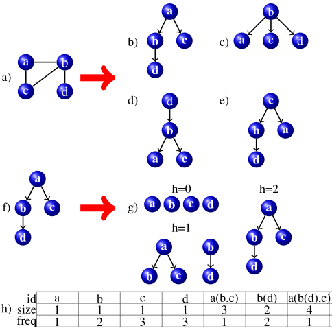
The set of features of a graph G are obtained as follows (see [Da San Martino et al., 2012] for details):
- ∀v ∈ V , perform a visit, i.e. a depth-first search, of G removing all the edges that would form a cycle. The result of the visit is a Directed Acyclic Graph (DAG). Figure 1a gives an example of a graph and Figure 1b-e the DAGs resulting from the visits.
- Given a parameter h, for each DAG obtained at the previous step, perform, from any node, an iterative deepening visit with limit h. Each visit generates a tree (a rooted connected directed acyclic graph where each node has at most one incoming edge). Figure 1f-g shows a DAG and the result of the iterative deepening visit for h = 2. Finally, any proper subtree of a tree T, i.e. the tree rooted at any node of T and comprising all of its descendants, is a feature. Figure 1h lists the contribution to the φ() of the DAG in subfigure f). The value of the feature f in φ(x) is its frequency of appearance multiplied by λ|f| , where |f| is the number of nodes composing the subtree f and λ is a user defined parameter.
Since each feature can be associated to a unique string, φ(x) can be compactly represented by a hash map (see Figure 1h). In [Da San Martino et al., 2012] it is shown that all the needed information is collected at once by performing (single) visits at depth h for each node of each graph in the dataset. Notice that, in order to exactly represent φ(x) in the primal version of the PA, we need to keep, for each feature, its hash key, frequency and size. Thus the memory occupancy of the φ() is 3|w|. In [Da San Martino et al., 2012] it is described a kernel function K(xt, xu) = φ(xt) · φ(xu), where φ() is the one described in this section. K() is defined on the input space and its computational complexity is O(|V | log |V |), where |V | is the number of nodes of G. If we consider the dual version of the PA, the memory occupancy of a graph G can be measured as |M| = |V |+|E|+1, where |E| the number of edges of G and 1 accounts for the τ value of the example.
Examples of other kernel functions whose φ() mapping support a sparse representation through a hash function can be found in [Shervashidze and Borgwardt, 2009; Costa and De Grave, 2010]
2.3 Lossy Counting
The Lossy Counting is an algorithm for computing frequency counts exceeding a user-specified threshold over data streams [Manku and Motwani, 2002]. Let s ∈ (0, 1) be a support threshold, ϵ ≪ s an error parameter, and N the number of items of the stream seen so far. By using only O ( 1ϵ log(ϵN)) space to keep frequency estimates, Lossy Counting, at any time N is able to i) list any item whose frequency exceeds ϵN; ii) avoid listing any item with frequency less than (s - ϵ)N. Moreover, the error of the estimated frequency of any item is at most ϵN.
In the following the algorithm is sketched, for more details refer to [Manku and Motwani, 2002]. The stream is divided into buckets Bi. The size of a bucket is |Bi| = ⌈ 1ϵ ⌉ items. Note that the size of a bucket is determined a priori because ϵ is a user-defined parameter.
The frequency of an item f in a bucket Bi is represented as Ff,i, the overall frequency of f is Ff = ∑i Ff,i. The algorithm makes use of a data structure D composed by tuples (f,Φf,i,∆i), where Φf,i is the frequency of f since it has been inserted into D, and ∆i is an upper bound on the estimate of Ff at time i.
The algorithm starts with an empty D. For every new event f arriving at time i, if f is not present in D, then a tuple (f, 1, i-1) is inserted in D, otherwise Φf,i is incremented by 1. Every |Bi| items all those tuples such that Φf,i +∆i ≤ i are removed.
The authors prove that, after observing N items, if f /∈ D then Φf,N ≤ ϵN and ∀(f, Φf,N , ∆N ).Φf,N ≤ Ff ≤ Φf,N + ϵN .
3 Our Proposal
In this section, we first propose a Lossy Counting (LC) algorithm with budget and able to deal with events weighted by positive real values. Then, we show how to apply the proposed algorithm to the Passive Aggressive algorithm in the case of a stream of graphs.
3.1 LCB: LCwith budget for weighted events
The Lossy Counting algorithm does not guarantee that the available memory will be able to contain the ϵ-deficient synopsis D of the observed items. Because of that, we propose an alternative definition of Lossy Counting that addresses this issue and, in addition, is able to deal with weighted events. Specifically, we assume that the stream emits events e constituted by couples (f, φ), where f is an item id and φ ∈ R+
is a positive weight associated to f. Different events may have the same item id while having different values for the weight, e.g. e1 = (f, 1.3) and e2 = (f, 3.4). We are interested in maintaining a synopsis that, for each observed item id f, collects the sum of weights observed in association with f. Moreover, we have to do that on a memory budget. To manage the budget, we propose to decouple the ϵ parameter from the size of the bucket: we use buckets of variable sizes, i.e. the i-th bucket Bi will contain all the occurrences of events which can be accommodated into the available memory, up to the point that D will use the full budget and no new event can be inserted into it. This strategy implies that the approximation error will vary according to the size of the bucket, i.e. ϵi = 1 |Bi| . Having buckets of different sizes, the index of the current bucket bcurrent is defined as bcurrent = 1 + maxk[∑ks=1 |Bs| < N]. Deletions occur when there is no more space to insert a new event in D. Trivially, if N events have been observed when the i-th deletion occurs, ∑is=1 |Bs| = N and, by definition, bcurrent ≤ ∑is=1 ϵs|Bs|.
Let φf,i(j) be the weight of the j-th occurrence of f in Bi, and the cumulative weight associated to f in Bi as wf,i = ∑Ff,i j=1 φf,i(j). The total weight associated to bucket Bi can then be defined as Wi = ∑f∈D wf,i. We now want to define a synopsis D such that, having observed N = ∑is=1 |Bs| events, the estimated cumulative weights are less than the true cumulative weights by at most ∑is=1 ϵiWi, where we recall that ϵi = 1 |Bi| . In order to do that we define the cumulated weight for item f in D, after having observed all the events in Bi, as Φf,i = ∑is=if wf,s, where if ≤ i is the largest index of the bucket where f has been inserted in D. The deletion test is then defined as
where ∆i = ∑is=1 Wi |Bi| . However, we have to cover also the special case in which the deletion test is not able to delete any item from D2 . We propose to solve this problem as follows: we assume that in this case a new bucket Bi+1 is created containing just a single ghost event (fghost, Φmin i -∆i), where fghost ̸∈ D and Φmin i = minf∈D Φf,i, that we do not need to store in D. In fact, when the deletion test is run, ∆i+1 = ∆i + Wi+1 |Bi+1| = Φmin i since Wi+1 = Φmin i -∆i and |Bi+1| = 1, which will cause the ghost event to be removed since Φghost,i+1 = Φmin i -∆i and Φghost,i+1+∆i = Φmin i . Moreover, since ∀f ∈ D we have Φf,i = Φf,i+1, all f such that Φf,i+1 = Φmin i will be removed. By construction, there will always be one such item.
Theorem 1. Let Φtrue f,i be the true cumulative weight of f after having observed N = ∑is=1 |Bs| events. Whenever an entry (f, Φf,i, ∆) gets deleted, Φtrue f,i ≤∆i.
2 E.g, consider the stream (f1, 10), (f2, 1), (f3, 10), (f4, 15), (f1, 10), (f3, 10), (f5, 1), .. and budget equal to 3 items: the second application of the deletion test will fail to remove items fromD.
Proof. We prove by induction. Base case: (f,Φf,1, 0) is deleted only if Φf,1 = Φtrue f,1 ≤ ∆1. Induction step: let i∗ > 1 be the index for which (f,Φf,i∗,∆) gets deleted. Let if < i∗ be the largest value of bcurrent for which the entry was inserted. By induction Φtrue f,if ≤ ∆if and all the weighted occurrences of events involving f are collected in Φf,i∗. Since Φtrue f,i∗ = Φtrue f,if + Φf,i∗ we conclude that Φtrue f,i∗ ≤∆if +Φf,i∗ ≤∆i∗.
Proof. If ∆ = 0 then Φf,i = Φtrue f,i . Otherwise, ∆ = ∆if , and an entry involving f was possibly deleted sometimes in the first if buckets. From the previous theorem, however, we know that Φtrue f,if ≤∆if , so Φf,i ≤ Φtrue f,i ≤ Φf,i +∆.
We notice that, if ∀e = (f, φ), φ = 1, the above theorems apply to the not weighted version of the algorithm.
Let now analyze the proposed algorithm. Let Oi be the set of items that have survived the last (i.e., (i - 1)-th) deletion test and that have been observed in Bi, Ii be the set of items that have been inserted in D after the last (i.e., (i - 1)-th) deletion test; notice that Oi ∪ Ii is the set of all the items observed in Bi, however it may be properly included into the set of items stored in D. Let wO i = ∑f∈Oi Ff,i and wI i = ∑f∈Ii Ff,i. Notice that wI i > 0, otherwise the budget would not be fully used; moreover, |Bi| = wO i + wI i . Let W O i = ∑f∈Oi wf,i and W I i = ∑f∈Ii wf,i. Notice that Wi = W O i +W I i , and that Wi |Bi| = wO i |Bi| [̂ W O i -̂ W I i ]+̂ W I i = pOi [̂ W O i -̂ W I i ]+̂ W I i , where pOi = wO i |Bi| is the fraction of updated items in Bi, ̂ W O i = W O i wO i is the average of the updated items, ̂ W I i = W I i wI i is the average of the inserted items. Thus Wi |Bi| can be expressed as a convex combination of the average of the updated items and the average of the inserted items, with combination coefficient equal to the fraction of updated items in the current bucket. Thus, the threshold ∆i used by the i-th deletion test can be written as
Combining eq. (3) with eq. (4) we obtain
If f ∈ Ii, then if = i and the test reduces to wf,i ≤ pOi [̂ W O i -̂ W I i ] +̂ W I i . If f ̸∈ Ii (notice that this condition means that if < i, i.e. f ∈ Iif ), then the test can be rewritten as wf,i ≤ pOi [̂ W O i -̂ W I i ]+̂ W I i - ∑i-1 s=if γf,s, where γf,s = wf,s - pOs [̂ W O s - ̂ W I s ] + ̂ W I s is the credit/debit gained by f for bucket Bs. Notice that, by definition, ∀k ∈ {if , . . . , i} the following holds ∑ks=if γf,s > 0.
3.2 LCB-PA on streams of Graphs
This section describes an application of the results in Section 3.1 to the primal PA algorithm. We will refer to the algorithm described in this section as LCB-PA. The goal is to use the synopsis D created and maintained by LCB to approximate at the best w, according to the available budget. This is obtained by LCB since only the most influential wi values will be stored into D.
A difficulty in using the LCB synopsis is due to the fact that LCB can only manage positive weights. We overcome this limitation by storing for each feature f in D a version associated to positive weight values and a version associated to (the modulus) of negative values.
Let's detail the proposed approach in the following. First of all, recall that we consider the features generated by the φ() mapping described in Section 2.2.
When a new graph arrives from the stream (line 3 of Algorithm 1), it is first decomposed into a bag of features according to the process described in Section 2.2. Then the score for the graph is computed according to eq. (1) (line 4 of Algorithm 1). If the graph is misclassified (the test on line 6 of Algorithm 1 is true), then the synopsis D (i.e., w) has to be updated. In this scenario, an event corresponds to a feature f of the current input graph G. The weight φf,i(j) of a feature f appearing for the j-th time in the i-th bucket Bi, is computed multiplying its frequency in the graph G with the corresponding τ value computed for G according to eq. (2), which may result in a negative weight. Φf,i is the weighted sum of all φf,i(j) values of the feature f since f has last been inserted into D. In this way, the LCB algorithm allows to maintain an approximate version of the full w vector by managing the feature selection and model update steps (lines 7-10 of Algorithm 1). In order to cope with negative weights, the structure D is composed by tuples (f, |f|,Φ+f,i ,Φ-f,i ), where Φ+f,i corresponds to Φf,i computed only on features whose graph G has positive classification (Φ-f,i is the analogous for the negative class). Whenever the size of D exceeds the budget B, all the tuples satisfying eq. (3) are removed from D. Here ∆i can be interpreted as the empirical mean of the τ values observed in the current bucket. Note that the memory occupancy of D is now 4|w|, where |w| is the number of features in D. The update rule of eq. (2) is kept. However, when a new tuple is inserted into D at time N, the ∆N value is added to the τ value computed for G. The idea is to provide an upper bound to the Φ+f,N , Φ-f,N values that might have been deleted in the past from D. Theorem 1 shows that indeed ∆N is such upper bound.
4 Experiments
In this section, we report an experimental evaluation of the algorithm proposed in Section 3.2 (LCB-PA), compared to the baselines presented in Section 2.1. Our aim is to show that the proposed algorithm has comparable, if not better, classification performances than the baselines while being much faster to compute.
4.1 Datasets and Experimental Setup
We generated different graph streams starting from two graph datasets available from the PubChem website (http://pubchem.ncbi.nlm.nih.gov): AID:123 and AID:109. They comprise 40, 876 and 41, 403 compounds. Each compound is represented as a graph where the nodes are the atoms and the edges their bonds. Every chemical compound has an activity score correlated to the concentration of the chemical required for a 50% growth inhibition of a tumor. The class of a compound is determined by setting a threshold β on the activity score. By varying the threshold a concept drift is obtained. Three streams have been generated by concatenating the datasets with varying β values: "Chemical1" as AID:123 β = 40, AID:123 β = 47, AID:109 β = 41, AID:109 β = 50; "Chemical2" as AID:123 β = 40, AID:109 β = 41, AID:123 β = 47, AID:109 β = 50; "Chemical3" as the concatenation of Chemical1 and Chemical2.
We generated a stream of graphs from the LabelMe dataset 3 , which is composed of images whose objects are manually annotated [Russell and Torralba, 2008]. The set of objects of any image were connected by the Delaunay triangulation [Su and Drysdale, 1996] and turned into a graph. Each of the resulting 5, 342 graphs belong to 1 out of 6 classes. A binary stream is obtained by concatenating i = 1..6 times the set of graphs: the i-th time only the graphs belonging to class i are labeled as positive, the others together forming the negative class. The size of the stream is 32, 052. We refer this stream as Image.
We considered as baseline Algorithm 1 in its Primal and Dual versions, both using the φ() mapping defined in Section 2.2. We compared them against the algorithm presented in Section 3.2 (LCB-PA in the following). A preliminary set of experiments has been performed to determine the best removal policy for the baselines and to select algorithm and kernel parameters (an extensive evaluation was beyond the scope of this paper). The best removal policy for Primal PA algorithm is the one removing the feature with lowest value in w. The best policy for the Dual PA removes the example with the lowest τ value. The C parameter has been set to 0.01, while the kernel parameters has been set to λ = 1.6, h = 3 for chemical datasets, and to λ = 1, h = 3 for the Image dataset.
4.2 Results and discussion
The measure we adopted for performance assessment is the Balanced Error Rate (BER). This measure is particularly well suited when the distribution of the data is not balanced. The BER can be calculated as BER = 12 ( fp tn + fp + fn fn + tp ), where tp, tn, fp and fn are, respectively, true positive, true negative, false positive and false negative examples. In order to increase the readability of the results, in the following we report the 1-BER values. This implies that higher values mean better performances. In our experiments, we sampled 1-BER every 50 examples. In Table 1 are reported, for each algorithm and budget, the average of the 1-BER values over the whole stream.
3 http://labelme.csail.mit.edu/Release3.0/browserTools/php/ dataset.php
| Budget | Dual | Primal | LCB-PA | PA (B=∞) | |
|---|---|---|---|---|---|
| Chemical1 | 10,000 25,000 50,000 75,000 100,000 | 0.534 0.540 0.547 - - | 0.629 0.638 0.642 0.643 0.644 | 0.608 0.637 0.644 0.644 0.644 | 0.644 (B = 182, 913) |
| Chemical2 | 10,000 25,000 50,000 75,000 100,000 | 0.535 0.541 0.546 - - | 0.630 0.638 0.642 0.644 0.644 | 0.610 0.638 0.644 0.645 0.645 | 0.644 (B = 182, 934) |
| Chemical3 | 10,000 25,000 50,000 75,000 100,000 | 0.532 0.542 0.549 - - | 0.640 0.652 0.658 0.660 0.661 | 0.601 0.643 0.658 0.660 0.661 | 0.661 (B = 183, 093) |
| Image | 10,000 25,000 50,000 75,000 100,000 | 0.768 0.816 0.822 - - | 0.845 0.846 0.846 0.846 0.845 | 0.855 0.853 0.852 0.852 0.852 | 0.852 (B = 534, 903) |
It is easy to see that the performances of the Dual algorithm are poor. Indeed, there is no single algorithm/budget combination in which the performance of this algorithm is competitive with the other two. This is probably due to the fact that support graphs may contain many features that are not discriminative for the tasks.
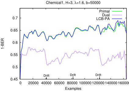
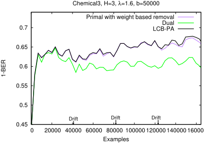
Let us consider the Primal and the LCB-PA algorithms. Their performances are almost comparable. Concerning the chemical datasets, Figure 2 and Figure 3 report the details about the performance of the Chemical1 stream. Similar plots can be obtained for Chemical2 dataset and thus are omitted. Figure 5 reports the performance plot on the Chemical3 stream with B = 50, 000. Observing the plots and the corresponding 1 - BER values, it's clear that on the three datasets the algorithm Primal performs better than LCB-PA for budget sizes up to 25, 000. For higher budget values, the performances of the two algorithms are very close, with LCB-PA performing better on Chemical1 and Chemical2 datasets, while the performances are exactly the same on Chemical3. Let's analyze in more detail this behavior of the algorithms. In Primal every feature uses 3 budget units, while in LCB-PA 4 units are consumed. In the considered chemical streams, on average every example is made of 54.56 features. This means that, with budget 10, 000, P rimal can store approximatively the equivalent of 60 examples, while LCB-PA only 45, i.e. a 25% difference. When the budget increases, such difference reduces. The LCB-PA performs better then the Primal PA with budget size of 50, 000 or more. Notice that LCB-PA, with budget over a certain threshold, reaches or improves over the performances of the PA with B = ∞.
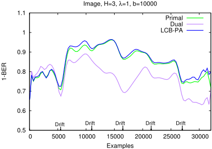
On the Image dataset we have a different scenario. LCB- PA with budget 10, 000 already outperforms the other algorithms.
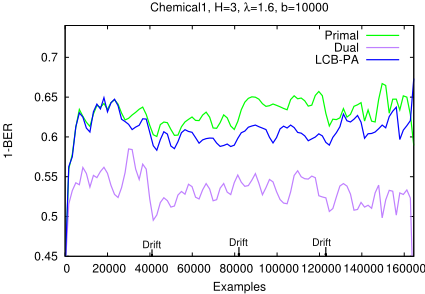
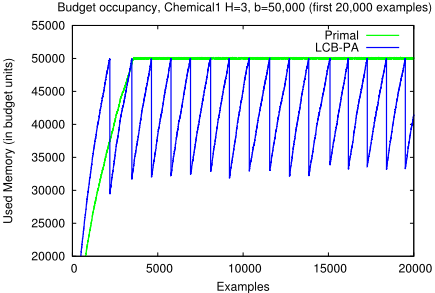
Table 2 reports the time needed to process the streams. It is clear from the table that LCB-PA is by far the fastest algorithm. Dual algorithm is slow because it works in the dual space, so it has to calculate the kernel function several times. The plot in Figure 4 reports the memory occupancy of Primal and LCB-PA algorithms. Notice that when the LCB-PA performs the cleaning procedure, it removes far more features from the budget then Primal. As a consequence, Primal calls the cleaning procedure much more often than LCB-PA, thus inevitably increasing its execution time. For example, on Chemical1 with budget 50, 000, Primal executes the cleaning procedure 132, 143 times, while LCB-PA only 142 times. Notice that a more aggressive pruning for the baselines could be performed by letting a user define how many features have to be removed. Such a parameter could be chosen a piori, but it would be unable to adapt to a change in the data distribution and there would be no guarantees on the quality of the resulting model. The parameter can also be tuned on a subset of the stream, if the problem setting allows it. In general, developing a strategy to tune the parameter is not straightforward and the tuning procedure might have to be repeated multiple times, thus increasing significantly the overall computational burden of the learning algorithm. Note that, on the contrary, our approach employs a principled, automatic way, described in eq. (4), to determine how many and which features to prune.
5 Conclusions and FutureWorks
This paper presented a fast technique for estimating the weighted frequency of a stream of features based on an extended version of Lossy Counting algorithm. It uses it for: i) pruning the set of features of the current solution such that it is ensured that it never exceeds a predefined budget; ii) prediction, when a feature not present in the current solution is first encountered. The results on streams of graph data show that the proposed technique for managing the budget is much faster than competing approaches. Its classification performance, provided the budget exceeds a practically very low value, is superior to the competing approaches, even when no budget constraints are considered for them.
| Chemical1 | Chemical2 | |||
|---|---|---|---|---|
| Budget | 10, 000 | 50, 000 | 10, 000 | 50, 000 |
| Dual | 5h44m | 31h02m | 5h42m | 31h17m |
| Primal | 44m19s | 1h24m | 43m54s | 1h22m |
| LCB-PA | 4m5s | 3m55s | 3m52s | 3m57s |
| Chemical3 | Image | |||
| Budget | 10, 000 | 50, 000 | 10, 000 | 50, 000 |
| Dual | 10h50m | 60h31m | 49m34s | 6h18m |
| Primal | 1h32m | 2h44m | 7m21s | 33m18s |
| LCB-PA | 7m41s | 7m45s | 0m49s | 0m50s |
As future work we intend to apply the proposed methodolgy to different domains, such as natural language processing and image analysis.
Acknowledgments
This work was supported by the Italian Ministry of Education, University, and Research (MIUR) under Project PRIN 2009 2009LNP494 005.
@inproceedings{ijcai2013p195,
  title     = {A Lossy Counting Based Approach for Learning on Streams of Graphs on a Budget},
  author    = {Martino, Giovanni Da San and Navarin, Nicolò and Sperduti, Alessandro},
  booktitle = {Proceedings of the Twenty-Third International Joint Conference on
               Artificial Intelligence, {IJCAI-13}},
  publisher = {AAAI Press / International Joint Conferences on Artificial Intelligence},
  editor    = {Francesca Rossi},
  pages     = {1294--1300},
  year      = {2013},
  month     = {8},
  url       = {https://ijcai.org/proceedings/2013/195},
}
TY - CPAPER TI - A Lossy Counting Based Approach for Learning on Streams of Graphs on a Budget AU - Martino, Giovanni Da San AU - Navarin, Nicolò AU - Sperduti, Alessandro T2 - Proceedings of the Twenty-Third International Joint Conference on Artificial Intelligence, IJCAI-13 PB - AAAI Press / International Joint Conferences on Artificial Intelligence PY - 2013 SP - 1294 EP - 1300 UR - https://ijcai.org/proceedings/2013/195 ER -Copied
Machine-readable versions of this paper, for tools and AI agents:





