
Exact Top-k Feature Selection via l2, 0-Norm Constraint
Proceedings of the Twenty-Third International Joint Conference on Artificial Intelligence. Pages 1240-1245.
© 2013 International Joint Conferences on Artificial Intelligence
Abstract
In this paper, we propose a novel robust and pragmatic feature selection approach. Unlike those sparse learning based feature selection methods which tackle the approximate problem by imposing sparsity regularization in the objective function, the proposed method only has one l2,1-norm loss term with an explicit l2,0-Norm equality constraint. An efficient algorithm based on augmented Lagrangian method will be derived to solve the above constrained optimization problem to find out the stable local solution. Extensive experiments on four biological datasets show that although our proposed model is not a convex problem, it outperforms the approximate convex counterparts and state of the art feature selection methods evaluated in terms of classification accuracy by two popular classifiers. What is more, since the regularization parameter of our method has the explicit meaning, i.e. the number of feature selected, it avoids the burden of tuning the parameter, making it a pragmatic feature selection method.
- [Argyriou et al., 2007] Andreas Argyriou, Charles A. Mic- chelli, Massimiliano Pontil, and Yiming Ying. A spectral regularization framework for multi-task structure learning. In NIPS, 2007.
- [Bertsekas, 1982] D.P. Bertsekas. Constrained optimization and lagrange multiplier methods. Computer Science and Applied Mathematics, Boston: Academic Press, 1982, 1, 1982.
- [Bertsekas, 1996] Dimitri P. Bertsekas. Constrained opti- mization and lagrange multiplier methods. Athena Sci- entific, 1996.
- [Cai et al., 2011] Xiao Cai, Feiping Nie, Heng Huang, and Chris H. Q. Ding. Multi-class l2, 1-norm support vector machine. In ICDM, pages 91-100, 2011.
- [Ding et al., 2006] Chris H. Q. Ding, Ding Zhou, Xiaofeng He, and Hongyuan Zha. R 1 -pca: rotational invariant l 1 - norm principal component analysis for robust subspace factorization. In ICML, pages 281-288, 2006.
- [Duda et al., 1995] R.O. Duda, P.E. Hart, and D.G. Stork. Pattern classification and scene analysis 2nd ed. 1995.
- S.P. Fodor. Massively parallel genomics. Sci- ence(Washington), 277(5324):393-395, 1997.
- [Forman and Kirshenbaum, 2008] George Forman and Evan Kirshenbaum. Extremely fast text feature extraction for classification and indexing. In CIKM, pages 1221-1230, 2008.
- [Guyon and Elisseeff, 2003] Isabelle Guyon and André Elis- seeff. An introduction to variable and feature selec- tion. Journal of Machine Learning Research, 3:1157- 1182, 2003.
- [Guyon et al., 2002] Isabelle Guyon, Jason Weston, Stephen Barnhill, and Vladimir Vapnik. Gene selection for can- cer classification using support vector machines. Machine Learning, 46(1-3):389-422, 2002.
- [Habbema and Hermans, 1977] JDF Habbema and J. Her- mans. Selection of variables in discriminant analysis by F-statistic and error rate. Technometrics, 19(4):487-493, 1977.
- [Hall and Smith, 1999] Mark A. Hall and Lloyd A. Smith. Feature selection for machine learning: Comparing a correlation-based filter approach to the wrapper. In FLAIRS Conference, pages 235-239, 1999.
- [Kira and Rendell, 1992] Kenji Kira and Larry A. Rendell. A practical approach to feature selection. In ML, pages 249-256, 1992.
- [Kohavi and John, 1997] Ron Kohavi and George H. John. Wrappers for feature subset selection. Artif. Intell., 97(1- 2):273-324, 1997.
- [Luo et al., 2010] Dijun Luo, Chris H. Q. Ding, and Heng Huang. Towards structural sparsity: An explicit l2/l0 ap- proach. In ICDM, pages 344-353, 2010.
- [Mancera and Portilla, 2006] Luis Mancera and Javier Por- tilla. L0-norm-based sparse representation through alter- nate projections. In ICIP, pages 2089-2092, 2006.
- [Nie et al., 2010] Feiping Nie, Heng Huang, Xiao Cai, and Chris H. Q. Ding. Efficient and robust feature selection via joint ;2, 1-norms minimization. In NIPS, pages 1813- 1821, 2010.
- [Nutt et al., 2003] C.L. Nutt, DR Mani, R.A. Betensky, P. Tamayo, J.G. Cairncross, C. Ladd, U. Pohl, C. Hart- mann, M.E. McLaughlin, T.T. Batchelor, et al. Gene expression-based classification of malignant gliomas cor- relates better with survival than histological classification. Cancer Research, 63(7):1602, 2003.
- [Obozinski et al., 2010] Guillaume Obozinski, Ben Taskar, and Michael I. Jordan. Joint covariate selection and joint subspace selection for multiple classification problems. Statistics and Computing, 20(2):231-252, 2010.
- [Peng et al., 2005] Hanchuan Peng, Fuhui Long, and Chris H. Q. Ding. Feature selection based on mutual infor- mation: Criteria of max-dependency, max-relevance, and min-redundancy. IEEE Trans. Pattern Anal. Mach. Intell., 27(8):1226-1238, 2005.
- [Powell, 1969] M. J. D. Powell. A method for nonlinear con- straints in minimization problems. In R. Fletcher, editor, Optimization. Academic Press, London and New York, 1969.
- [Raileanu and Stoffel, 2004] Laura Elena Raileanu and Kil- ian Stoffel. Theoretical comparison between the gini in- dex and information gain criteria. Ann. Math. Artif. Intell., 41(1):77-93, 2004.
- [Saeys et al., 2007] Yvan Saeys, Iñaki Inza, and Pedro Larrañaga. A review of feature selection techniques in bioinformatics. Bioinformatics, 23(19):2507-2517, 2007.
- [Singh et al., 2002] D. Singh, P.G. Febbo, K. Ross, D.G. Jackson, J. Manola, C. Ladd, P. Tamayo, A.A. Renshaw, A.V. D'Amico, J.P. Richie, et al. Gene expression cor- relates of clinical prostate cancer behavior. Cancer cell, 1(2):203-209, 2002.
- [Su et al., 2001] A.I. Su, J.B. Welsh, L.M. Sapinoso, S.G. Kern, P. Dimitrov, H. Lapp, P.G. Schultz, S.M. Powell, C.A. Moskaluk, H.F. Frierson, et al. Molecular classifica- tion of human carcinomas by use of gene expression sig- natures. Cancer Research, 61(20):7388, 2001.
- [Wang et al., 2011] H Wang, F Nie, H Huang, S L Risacher, C Ding, A J Saykin, L Shen, and ADNI. A new sparse multi-task regression and feature selection method to iden- tify brain imaging predictors for memory performance. ICCV 2011: IEEE Conference on Computer Vision, pages 557-562, 2011.
References were extracted automatically from the PDF and may contain errors.
Full text extracted automatically from the PDF; figures, tables and equations may differ. The PDF is the version of record.
1 Introduction
Feature selection primarily addresses the problem of finding the most relevant and informative set of features. Besides that, it can have other motivations, including general data compression, to reduce the size of the data when the data is huge and the data storage space is limited; performance enhancement, to improve the prediction accuracy and boost the model generalization capability; data understanding, to gain knowledge about the process that generated the data or simply visualize the data; processing acceleration, to decrease the algorithm running time in the real application. As we know, high-dimensional data in the input space is usually not good for classification due to the curse of dimensionality. Although we can employ the traditional dimension reduction method, i.e. PCA, LDA and etc., to reduce the feature size, we cannot tackle the problems where the features have natural meanings and they cannot be projected, such as text mining [Forman and Kirshenbaum, 2008],to select text key words; DNA
∗Corresponding Author. This work was partially supported by NSF CCF-0830780, CCF-0917274, DMS-0915228, IIS-1117965.
microarray [Peng et al., 2005], to find out a few of genes associated with a given disease; mass spectrometry [Saeys et al., 2007], to discover the protein-based biomarker profiling [Saeys et al., 2007]. Therefore, feature selection is an essential component of machine learning and data mining and a large number of developments on feature selection have been made in the literature [Guyon and Elisseeff, 2003].
Generally speaking, feature selection algorithms may roughly be categorized into three main families: filter, wrapper and embedded methods. These three basic categories differ in how the learning algorithm is incorporated in evaluating and selecting features. In filter methods, features are pre-selected by the intrinsic properties of the data without running the learning algorithm. Therefore, filter methods are independent of the specific learning algorithm and can be characterized by utilizing the global statistical information. Popular filter-type feature selection methods encompass F-statistic [Habbema and Hermans, 1977], reliefF [Kira and Rendell, 1992], mRMR [Peng et al., 2005], t-test, Chi-square and information gain [Raileanu and Stoffel, 2004] and etc., which all compute the sensitivity (correlation or relevance) of a feature with respect to (w.r.t.) the class label distribution of the data. In wrapper methods [Kohavi and John, 1997], the process of feature selection is wrapped around the learning algorithm that will ultimately be employed and take advantage of the "feedbacks" from the learning algorithm, such as correlation-based feature selection (CFS) [Hall and Smith, 1999], support vector machine recursive feature elimination (SVMRFE) [Guyon et al., 2002]. In spite of expensive computational cost, they often have good performance. In embedded methods, feature search and the learning algorithm are incorporated into a single optimization problem, such that the reasonable computational cost can be achieved for good classification performance. Thus, the embedded methods have attracted large attention in data mining and machine learning research societies.
Recently, with the development of sparsity research, both theoretical and empirical studies have suggested that the sparsity is one of the intrinsic properties of real world data and sparsity regularization has been applied into embedded feature selection models as well. In multi-task learning, Argyriou et. al. has developed a multi-task feature learning method [Argyriou et al., 2007]. Specifically, when the rotation matrix U equals to an identity matrix, that feature learning model is equivalent to using a least square loss function with a ℓ2,1-norm square regularization term. Therefore, such regularization has close connection to group LASSO and can couple feature selection across multiple tasks. According to the structure of the norm, the sparsity can be obtained from the following two types of regularization terms for feature selection: Flat sparsity, where the sparsity is often achieved by ℓ1-norm or ℓ0-norm regularizer to select individual feature; Structural sparsity, where the ℓ2,1-norm, ℓ2,∞-norm or ℓ2,0norm are imposed to select group features.
Since we are focusing on multi-class feature selection, structured sparsity regularization is desired, which can select the features across all the classes with jointly sparsity, i.e. each feature has either small score or large score for all the classes. From the sparsity perspective, although ℓ2,0norm is more desirable, due to its non-convex and nonsmooth properties which will induce great difficulty in optimization, people prefer the convex ℓ2,1-norm as the regularization term [Nie et al., 2010; Cai et al., 2011; Wang et al., 2011]. As we know, such kind of approximation is under the assumption that the effects of ℓ2,0-norm regularization is identical or approximately identical to the ℓ2,1-norm. Nevertheless, the above assumption does not always hold in the real application [Mancera and Portilla, 2006]. Moreover, since the regularization parameter of ℓ2,1-norm does not have explicit meaning, for different data, it may change dramatically and people need to carefully tune its value based on the training data, which will take long time. Lots of related work of sparse learning based feature selection methods adopt the model based on convex problem due to the fact that convex problem has global solution. However, is it always true that the method based on convex problem is always better than that based on non-convex problem?
In this paper, we will propose an efficient, robust, and pragmatic multi-class feature selection model, which has the following advantages: (1) We show that it is NOT true that the feature selection method based on convex problem is always better than its counterpart based on non-convex problem. (2) We tackle the original sparse problemwith ℓ2,0-norm constraint directly instead of its relaxation or approximation problem. Therefore, we can get a more accurate solution. (3) Since there is only one term in the objective function, we avoid the computational burden of tuning the parameter for regularization term, which is desired for solving the real problem. (4) We are the first to provide an efficient algorithm to tackle the minimization problem of ℓ2,1-norm loss with the ℓ2,0-norm constraint. Extensive experiments on four benchmark biological datasets show that our approach outperforms the relaxed or approximate counterparts and state-of-art feature selection methods evaluated in terms of classification accuracy using two popular classifiers.
Notation. We summarize the notations and the definition of norms used in this paper. Matrices are written as uppercase letters and vectors are written as bold lowercase letters. For matrix W = {wij}, its i-th row, j-th column are denoted as wi , wj respectively. The ℓp-norm of the vector v ∈ Rn is defined as ‖v‖p = ( n∑ i=1 |vi|p ) 1p , for p ̸= 0 and the ℓ0-norm of the vector v, is defined as the number of non-zero entries of v. The Frobenius norm of the matrix W ∈ Rd×m is defined as ‖W‖F = √ d∑ i=1 m∑ j=1 w2 ij = √ d∑ i=1 ‖wi‖22 . And the ℓ2,1-norm of matrix W is defined as |W||2,1 = d∑ i=1 √ m∑ j=1 w2 ij and the ℓ2,0-norm of matrix W is defined as ||W||2,0 = d∑ i=1 || m∑ j=1 w2 ij ||0, where for a scalar a, ||a||0 = 1 if a ̸= 0, ||a||0 = 0 if ||a|| = 0. Please note that ℓ2,0-norm is not a valid norm because it does not satisfies the positive scalability: ||αW||2,1 = |α|||W||2,1 for any scalar α. The term "norm" here is for convenience.
2 Sparse Learning Based Feature Selection Background
Typically, many sparse based supervised binary feature selection methods that arise in data mining and machine learning can be written as the approximation or relaxed version of the following problem:
where y ∈ Bn×1 is the binary label, X ∈ Rd×n is the training data, w ∈ Rd×1 is the learned model, b is the learned biased scalar, 1 ∈ Rn×1 is a column vector with all 1 entries, and k is the number of the feature selected. Solving Eq. (1) directly has been approved NP-hard, very difficult in optimization. In many practical situations it is convenient to allow for a certain degree of error, and we can relax the optimization constraint using the following formulation,
which is equivalent to the following "fidelity loss plus regularization" format,
where λ ∈ R+ is the regularization parameter. Unfortunately, the way to tackle Eq. (3) is still challenging. To overcome this problem, the subsequent alternative formulation using ℓ1norm regularization instead of ℓ0-norm has been proposed,
After we get w∗ , we choose the feature indices corresponding to top k largest values of the summation of absolute values along each row. In statistic, people call Eq. (4) as the regularized counterpart of LASSO problem, which has been widely studied and proved to have a closed form solution.
Although people can use heuristic strategy, i.e. one V.S. all or one V.S. one to extend the above binary sparse based feature selection method to do multi-class feature selection, some structural sparsity is preferred, if the goal is to select features across all the classes. In multi-task learning, Obozinsky et al. and Argyriou et. al. [Argyriou et al., 2007] [Obozinski et al., 2010] have developed a ℓ2,1-norm square regularization term to couple feature selection across tasks.
3 Robust and Pragmatic Multi-class Feature Selection
Given training data {x1, x2, · · · , xn} ∈ Rd×1 and its corresponding class labels {y1, y2, · · · , yn} ∈ Rm×1 , traditional least square regression solves the following optimization problem to learn the projection matrix W ∈ Rd×m and the bias b ∈ Rm×1 :
Since there is inevitable noise existing in the training data, in order to be robust to outliers, our proposed method will use the robust loss function:
which has a rotational invariant property whereas the pure ℓ1norm loss function does not has such desirable property [Ding et al., 2006]. In addition, for the sake of obtaining a more accurate model, we use ℓ2,0-norm constraint instead of impose it as the regularization term.
Denoting n training data X ∈ Rd×n as well as the associated class labels Y ∈ Rn×m for m classes, in this paper, we propose the following objective function to select k features in multi-class problems
where, 1 ∈ Rn×1 is a column vector with all its entries being 1.
4 Optimization Algorithm
In this section, we will propose an efficient algorithm to tackle Eq. (7) directly followed by the proof of its convergence to local solution.
4.1 General Augmented LagrangianMultiplier Method
In [Bertsekas, 1982], the general method of augmented Lagrange multipliers is introduced for solving constrained optimization problems of the kind:
One may define the augmented lagrangian function:
where matrix Λ is the Lagrange multiplier and µ is a positive scalar called the quadratic penalty parameter and then Eq. (9) can be solved via the method of augmented Lagrange multipliers, outlined as Alg. 1.
4.2 ProblemReformulation
According to Augmented Lagrangian Multiplier (ALM) Method, we introduce two slack variables i.e. V and E. Eq. (7) can be reformulated as
4.3 An Efficient Algorithm to Solve the Constrained Problem
We will introduce an efficient algorithm based on the general ALM to tackle problem Eq. (10) alternatively and iteratively.
The first step is fixing W, V and E, solving b. Then we need to solve the following subproblem:
Take derivative w.r.t. b and set it to zero, we have
The second step is fixing V , b and E, solving W. Then the objective function becomes,
Take derivative w.r.t. W and set it to zero, we have
where I ∈ Rd×d is the identity matrix.
The third step is fixing W, b and E, solving V . The subproblem becomes,
which can be solved by Alg. 2.
The fourth step is fixing W, b and V , solving E. The subproblem becomes,
Denote
Then Eq. (16) is equivalent to the following problem,
which can be decoupled as,
Algorithm 1 General Method of Augmented Lagrange Multiplier
Initialization:
- Set t = 0
- Initialize the Lagrangian multiplier matrix Λ(t) .
- Initialize the quadratic penalty parameter µ(t) .
- Initialize the incremental step size parameter ρ ≥ 1.
repeat
- Update X(t+1) = arg min L(X(t) , Λ(t) , µ(t) )
X
- Update Λ(t+1) = Λ(t) + µ(t)h(X(t+1) )
- Update µ(t+1) = ρµ(t)
- Update t = t + 1
until Converges
Output: X∗
Algorithm 2 The algorithm to solve Eq. (15)
Input:
- The projection matrix W.
- The Lagrangian multiplier matrix Λ
- The quadratic penalty parameter µ.
- The number of feature selected k.
Process:
- Calculate ˜ W =W + 1µ Λ.
- Calculate the vector p ∈ Rd×1 , where each entry defined as
- pi = ∑j abs( ˜ wij), ∀i = 1, 2, · · · , d.
- Sort p, find out the indices vector q = [q1, q2, · · · , qk]T corresponding to top k sorted entries.
- Assign i-th row of ˜ W to V if i ∈ q; assign zero row vector 0T ∈ R1×mto V , if i /∈ q. Output: The slack variable matrix V .
where ei and gi is the i-th row of matrix E and G respectively. And the solution to Eq. (19) is
We iteratively and alternatively update b,W, V, E according to the above four steps and summarize the whole Algorithm in Alg. 3.
4.4 AlgorithmAnalysis
Since Eq. (10) is not a convex problem, in each iteration, given fixed Λ, Σ, and µ, Alg. 3 will find its local solution. The convergence of ALM algorithm was proved and discussed in previous papers. Please refer to the literature therein [Bertsekas, 1996] [Powell, 1969].
The overall computation complexity of our method is low, although we solve it separately and iteratively. In each iteration, the only computation burden is in Eq. (14), where we need to calculate an inverse d × d matrix. However, since it is only related to the input data, we can calculate it before we go to the loop. What is more, when the number of feature is much larger than the number of data, we can resort to Woodbury formula to transform it as a n × n inverse matrix. Although its solution depends on the initialization, in the following experiment section, we will conduct experiment to
Algorithm 3 The algorithm to solve Eq. (10)
Input:
- Training data Xtr ∈ Rd×ntr , training labels Ytr ∈ Rntr×m
- The number of feature selected k.
- The initial projection matrix W0.
Output:
- The k selected feature indices vector q.
- The objective function value obj
- The learned projection matrix W and bias b.
Initialization:
- Set t = 0
- Initialize the projection matrix as W = W0.
- Initialize the Lagrangian multiplier matrix Λ ∈ 0d×m, Σ ∈ 0n×m.
- Initialize the quadratic penalty parameter µ = 0.1.
- Initialize the incremental step size parameter ρ = 1.02.
Process:
repeat
- Update the bias b by Eq. (12).
- Update the projection matrix W by Eq. (14).
- Update the the slack variable matrix V by Alg. 2.
- Calculate G by Eq.(17).
- Update E by Eq. (20).
- Update Λ(t+1) = Λ(t) + µ(t) (W (t+1) - V (t+1) )
- Update Σ(t+1) = Σ(t) + µ(t) (XT W (t+1) + 1b(t+1)T - Y -E(t+1) )
- Update µ(t+1) = ρµ(t)
- Update t = t + 1
until Converges
| data name | # samples | # features | # classes |
|---|---|---|---|
| LEU | 72 | 3571 | 2 |
| LUNG | 203 | 3312 | 5 |
| ALLAML | 72 | 7129 | 2 |
| CAR | 174 | 9182 | 11 |
demonstrate that its local solution is stable and its feature selection performance is better than that of some state-of-art sparse feature selection methods based on convex problems.
5 Experiment
We denote our proposed method as ℓ2,0-norm ALM. The performance of ℓ2,0-norm ALM is evaluated on four biological gene expression datasets. We give a brief description of all datasets used in our subsequent experiments.
5.1 Datasets Descriptions
The gene expression datasets are the leukemia (LEU) data set [Nutt et al., 2003], the human lung carcinomas (lUNG) data set [Singh et al., 2002], ALLA data set [Fodor, 1997] and Human Carcinomas (Carcinomas) data set [Su et al., 2001]. All these four datasets are standardized to zero-mean and normalized by the standard deviation, which are summarized in Table 1.
LEU data set encompasses two classes samples: 25 leukemia patient (Positive), 47 healthy patient (Negative). Each sample has 3571 genes. Genes with minimal variations across the samples were removed before the experiment. Also, intensity thresholds were set at 20 and 16, 000 units for this data set. After preprocessing, we obtained a data with 72 samples and 3571 genes.
LUNG data contains 203 samples of five classes, which have 139, 21, 20, 6, 17 samples, respectively. Each sample has 12600 genes. In the preprocessing, the genes with standard deviations less than 50 expression units were removed and we got a data set with 203 samples and 3312 genes at last.
ALLA data set contains 72 samples of two classes, that is, ALL and AML, which have 47 and 25 samples, respectively. Each sample contains 7, 129 genes.
Carcinomas (CAR)data set is composed of 174 samples of eleven classes, prostate, bladder/ureter, breast, colorectal, gastroesophagus, kidney, liver, ovary, pancreas, lung adenocarcinomas and lung squamous cell carcinoma, which have 26, 8, 26, 23, 12, 11, 7, 27, 6, 14, 14 samples, respectively. The raw data encompasses 12533 genes and the after preprocessing, the data set has 174 samples and 9182 genes.
5.2 Experiment Setup
In our experiments, for each data, we will randomly select 20% to do the training and use the remaining part as testing. The reason we use smaller portion of training data is because it is well known that when the number of training data becomes sufficiently large, any feature selection method will work well. We select the number of features ranging from 1 to 10 with the incremental step 1 and the feature selection performance is evaluated by average classification accuracy on two popular classifiers, i.e. K nearest neighbor (KNN)
and support vector machine (SVM). Specifically, we set up KNN with K = 1 and SVM with linear kernel C = 1 respectively for their intuitive meaning and simplicity. Here we assume that the better the feature selection algorithm is, the higher classification accuracy we will get. We compare our feature selection method with the following two basic filter methods:
Fisher Score [Duda et al., 1995] selects each feature independently according to the score under the Fisher criterion.
Information Gain (IG) [Raileanu and Stoffel, 2004] computes the sensitivity (correlation or relevance) of a feature w.r.t the class label distribution of the data.
In addition, we also compare our approach with some similar feature selection methods based on sparse learning:
Multi-Task Feature Selection (MTFS) [Argyriou et al., 2007] selects features across multi-task (multi-class) by solving a general loss function with ℓ2,1-norm regularization. .
Robust Feature Selection (RFS) [Nie et al., 2010] selects features w.r.t multi-class and can be robust to the outlier data by solving a joint ℓ2,1-norm problem.
Sparse Feature Selection (SFS) [Luo et al., 2010] selects features by solving a smoothed general loss function with a more sparse ℓ2,0-norm constraint.
We tune the regularization parameter in MTFS and RFS to let the non-zero row number of the optimum solution W exactly equal to the number of selected features. Because MTFS and RFS both solve a convex optimization problem, they will get global solution finally. However, SFS and our method are based on ℓ2,0-norm constraint and we can only find local solution. In our experiment, we used the optimum solution of MTFS as the initialization for SFS and used random initialization for our method. Since there is an explicit meaning of the constraint k in our method or SFS, we can avoid the heavy burden of tuning regularization parameter and just make them as the number of selected features. We use the following parameters µ = 0.01, ρ = 1.02 and choose 1000 as the maximum number of iterations in Alg. 3.
| data | k = 1 | k = 5 | k = 8 | k = 10 |
|---|---|---|---|---|
| LEU | 1.72±1.80 | 0.68±0.49 | 0.58±0.43 | 0.66±0.37 |
| LUNG | 23.61±2.87 | 11.81±0.38 | 11.31±0.84 | 10.12±0.74 |
| ALLA | 6.06±2.26 | 2.45±1.24 | 1.28±0.85 | 0.92±0.56 |
| CAR | 29.69±1.73 | 23.01±1.70 | 19.81±1.68 | 18.40±1.48 |
5.3 Feature Selection Results
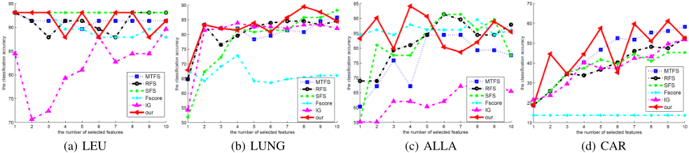
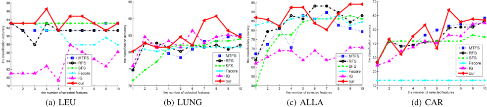
Fig. 1 shows the classification accuracy V.S. the number of selected feature using KNN classifier. Similarly, Fig. 2 demonstrates the feature selection results by SVM. From them, we can see that when the number of selected feature is small, particularly the one with less than 5 features, the classification result of our method can beat MTFL as well as RFS consistently, since our method can find a more sparse solution by ℓ2,0-norm constraint instead of the solution to the relaxed regularization problem. Because SFS finds local solution, its performance depends on the initialization, i.e. MTFS. When feature selection result of MTFS is good, like LEU data, SFS can achieve very promising results. However, for some data, like LUNG, when MTFS performs badly, SFS will stuck at the bad local optimum. When the number of selected feature increases, all the sparse learning based feature selection methods will tend to perform similarly, which is within our expectation. Next we will conduct experiment to show that our method can find stable local solutions under different random initializations.
5.4 Is The Local Solution Stable?
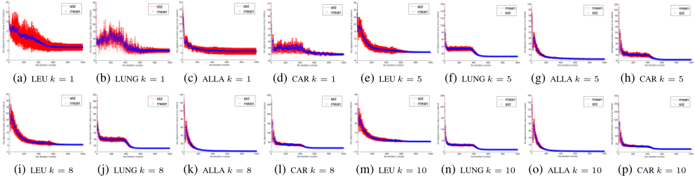
Since our proposed method in Eq. (7) is not a convex problem, we can only find the local optimum solution. We want to see if those local optimums are stable or not using different initialization. To be specific, each time when we run ℓ2,0norm ALM by Alg. 3, we use random initialization for the projection matrix W ∈ Rd×m as the input to do the training. We repeat 50 times experiment for each data and record the objective function value for each iteration. Fig. 3 plots the mean marked as blue circle as well as standard deviation marked as red error bar of the objective function value for each iteration using different initialization. For ease of comparison, we also list the converged mean and standard deviation value after converged in Table 2 when k = 1, k = 5, k = 8 and k = 10 respectively. As can be observed, our method will converge to a stable value using random initialization w.r.t. different number of selected features. Moreover, the larger number of feature (k) we selected, the less standard deviation (more stable) of the objective function value will be after it converges.
6 Conclusion
In this paper, we propose a robust and efficient feature selection approach to tackle an optimization problem with nonsmoothed ℓ2,1-norm loss function under ℓ2,0-norm constraint. The ℓ2,1-norm loss function can be robust to outlier data and ℓ2,0-norm constraint has an explicit meaning i.e. the number of selected features. Instead of solving its relaxed regularization problem, we tackle the constraint problem itself by taking advantage of ALM method. Thus, we can avoid the heavy burden of tuning regularization parameters and make it a practical feature selection method in the real life.
@inproceedings{ijcai2013p187,
  title     = {Exact Top-k Feature Selection via l2, 0-Norm Constraint},
  author    = {Cai, Xiao and Nie, Feiping and Huang, Heng},
  booktitle = {Proceedings of the Twenty-Third International Joint Conference on
               Artificial Intelligence, {IJCAI-13}},
  publisher = {AAAI Press / International Joint Conferences on Artificial Intelligence},
  editor    = {Francesca Rossi},
  pages     = {1240--1245},
  year      = {2013},
  month     = {8},
  url       = {https://ijcai.org/proceedings/2013/187},
}
TY - CPAPER TI - Exact Top-k Feature Selection via l2, 0-Norm Constraint AU - Cai, Xiao AU - Nie, Feiping AU - Huang, Heng T2 - Proceedings of the Twenty-Third International Joint Conference on Artificial Intelligence, IJCAI-13 PB - AAAI Press / International Joint Conferences on Artificial Intelligence PY - 2013 SP - 1240 EP - 1245 UR - https://ijcai.org/proceedings/2013/187 ER -Copied
Machine-readable versions of this paper, for tools and AI agents:





