Semiring-Based Mini-Bucket Partitioning Schemes

1 Introduction

The graphical model framework provides a common formalism to model complex systems such as probabilistic models, which includes Markov and Bayesian networks [Pearl, 1988], and deterministic models, which includes constraint networks [Bistarelli et al., 1999] and decision diagrams [Dechter, 2003]. In general, a graphical model is defined by a collection of functions or factors F over a set of variables X . Factors return values from a valuation set A. Depending on each particular case, functions may express probabilistic, deterministic or preferential information. Given a graphical model, one can compute different reasoning tasks. A reasoning task is defined by two operators ⊕ and ⊗, where the triplet (A,⊕,⊗) constitutes a semiring.

Since the exact computation of reasoning tasks is in general intractable, several approximation methods exist. Some of them need to solve internally an optimization problem over the set of partitions of a set of factors. Although it is known that the quality of the approximation depends greatly on the quality of the partitions, little research has been done on it.

This paper builds on top of the recent work of [Rollon and Dechter, 2010], where a greedy scheme is proposed for solving the partitioning problem of the very specific task of computing the probability of certain evidence. Our paper generalizes the partitioning problem and the greedy scheme to general tasks on graphical models. We show that the generalization applies as long as the semiring admits a division operator and a refinement of its order, which is the most usual case. Furthermore, we show the potential of this general partitioning scheme on the task of finding the most probable explanation of probabilistic networks.

2 Preliminaries

2.1 Semirings

A commutative semiring [Kohlas and Wilson, 2008] is a triplet (A, ⊕, ⊗), where A is a set, and ⊕, ⊗ are binary operations. Both operatios are associative and commutative. Additionally, ⊗ distributes over ⊕ (i.e, (a ⊗ b) ⊕ (a ⊗ c) = a⊗(b⊕c)). Commutative semirings have a unique 0 element such that 0 ⊗ a = 0. Additionally, they implicitely define a pre-order relation ≤ as a ≤ b (i.e., b is better than a) iff a = b or there exists c ∈ A such that a ⊕ c = b. In this paper we will restrict ourselves to semirings whose pre-order is a partial order.

Proposition 1 For any semiring (A, ⊕, ⊗), its associated relation ≤ satisfies:

1. a ≤ b and c ≤ d implies a⊗ c ≤ b ⊗d.
2. a⊗ b ≤ c ⊗ b implies a ≤ c.

In this paper we will consider invertible semirings [Kohlas and Wilson, 2008; Bistarelli and Gadducci, 2006; Cooper and Schiex, 2004; Lauritzen and Jensen, 1997], for which a division operation a c b exists. Division satisfies that for all a, b ∈ A such that a ≤ b and a ̸= 0, (a c b) ⊗ b = a. When a ≤ b and a = 0, we follow the approach in [Cooper and Schiex, 2004] and define 0 c b = 0.

Universitat Polit`

2.2 Factors

Let X = (x1, . . . , xn) be an ordered set of variables and D = (D1, . . . ,Dn) an ordered set of domains, where Di is the finite set of potential values for xi. DX is the set of possible assignments of X. Tuples are assignments of domain values to some or all the variables. The join of two tuples t and s is noted t · s.

A factor [Darwiche, 2009; Kask et al., 2005] f with scope Y ⊆ X is a function f : DY → A, where A is a semiring. The evaluation of factor f on tuple t will be noted f(t). If t assigns more variables than needed, they will be ignored. The scope of factor f will be denoted var(f).

The semiring order can also be extended to factors: f ≤ h iff ∀t ∈ Dvar(f)∪var(h), f(t) ≤ h(t). Note that this is a very coarse partial ordering. It requires the outcome of every tuple to be ordered. It may be the case of a function being almost always smaller than another and yet the partial order will not be able to discriminate between them.

Operations over valuations can be extended to functions:

• The combination of two functions f and g, noted f ⊗ g, is a new function with scope var(f) ∪ var(g) such that, ∀t ∈ Dvar(f)∪var(g), (f ⊗ g)(t) = f (t) ⊗ g(t).
• The division of two functions f and g such that ∀t ∈ Dvar(f)∪var(g), f(t) ≤ g(t), noted f ˆ g, is a new function with scope var(f) ∪ var(g) such that, ∀t ∈ Dvar(f)∪var(g), (f ˆ g)(t) = f (t) c g(t).
• The marginalization of f over x ∈ var(f), noted f ⇓x, is a function whose scope is var(f) - {x} such that, ∀t ∈ Dvar(f)-{x}, (f ⇓x)(t) = ⊕v∈Dx (t · v).

2.3 Graphical Models and Reasoning Tasks

A graphical model is a set of factors F over a set of variables X with domains D. A reasoning task is defined by P = (X,D,A,F, ⊕, ⊗) where (X,D,F) is a graphical model and (A, ⊕, ⊗) is a semiring. Computing the reasoning task means computing (⊗f∈F f) ⇓x1,x2,...,xn .

Example 1 In probabilistic graphical models valuations are probabilities (i.e, A = [0, 1]), the ⊗ operation is the product and the c operation is the division. For the reasoning task of finding the probability of evidence, the ⊕ operation is the sum. For the reasoning task of finding the most probable explanation, the ⊕ operation is the maximum.

In standard constraint networks we have boolean valuations (i.e, A = {true, false}), the ⊗ operation is the conjunction ∧ and the c operation is also the conjunction ∧. For the reasoning task of finding solutions, the ⊕ operation is the disjunction ∨. For the reasoning task of counting solutions, the ⊕ operation is the sum.

In weighted constraint networks valuations are natural numbers with infinity (i.e., A = N ∪ {∞}), the ⊗ operation is the sum and the c is the substraction. For the reasoning task of finding optimal solutions, the ⊕ operation is the minimum. For the reasoning task of counting weighted solutions, the ⊕ operation is the sum.

3 The Partitioning Problem

Computing reasoning tasks is in general intractable. Thus, several approximation methods have been proposed. Some of them (such as mini-bucket elimination [Dechter and Rish, 2003] or join-graph propagation algorithms [Mateescu et al., 2010]) require the computation of a good partition out of a set of factors, as described in the following.

A bucket B is a set of factors, all of which have a certain variable x in their scope. The scope of the bucket is the set of all variables in the scopes of its factors. The bucket function is,

Let Q = {Q1, Q2, . . . , Qk} be a partition of bucket B. Each partition element is called a mini-bucket. We say that Q is a z-partition if the scope size of all its mini-buckets is smaller than or equal to z. The function of partition Q is,

The rationale of the approximation is that µQ is likely to resemble µ, while being computationally simpler. More precisely, if Q is a z-partition, the cost of computing µQ is, at most, exponential in z. Approximation algorithms replace the bucket function by a function of one partition, for a fixed parameter z. Thus, it is of utmost importance finding the zpartition whose function resembles µ as much as possible.

3.1 The Partitions Lattice

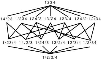
Given a bucket B, the set of all its partitions can be arranged as a lattice [Rollon and Dechter, 2010]. There is an upward edge from Q to Q′ if Q′ results from merging two minibuckets of Q in which case Q′ is a child of Q. The set of all children of Q is denoted by ch(Q). The bottom partition in the lattice, noted Q⊥, is the partition where every minibucket consists of a single function, while the top partition, noted Q⊤, is the partition with one mini-bucket containing all functions. Note that Q⊤ is equivalent to the whole bucket.

Example 2 Figure 1 depicts the partitioning lattice of bucket B = {f1, f2, f3, f4}. Its bottom partition Q⊥ is {{f1}, {f2}, {f3}, {f4}}, while its top partition Q⊤ is {{f1, f2, f3, f4}}. Partition Q = {{f1, f2}, {f3, f4}} is a child of partition Q′ = {{f1}, {f2}, {f3, f4}} because Q merges mini-buckets {f1} and {f2} in Q′ . However, Q is not a child of partition {{f1}, {f3}, {f2, f4}}.

Clearly, the set of z-partitions, for a given z, divides the lattice in two regions: the bottom region contains the zpartitions whose implicit function can be efficiently computed and the top bottom contains the rest of partitions whose implicit function is expensive.

There is a clear relation between lattice edges and the partial order of the partition's implicit functions.

Theorem 1 [Dechter and Rish, 2003; Bistarelli et al., 1997] Given two partitions Q and Q′ of bucket B, if Q′ is a descendent of Q then µQ′ ≤ µQ.

The previous theorem indicates that following any bottomup path the implicit functions decrease monotonically. Thus, as we follow the path, we obtain better approximations of the bucket function µ. Thus, given z, the low region of the lattice corresponds to more dissimilar functions, while the high region corresponds to more similar functions.

It is worth to mention that the lattice edges does not explicit all the orders among implicit functions. Some functions from different paths may also be ordered by the partial order although their partitions are not upward connected in the lattice.

3.2 Similarity Functions

The division allows us to capture how similar two functions are. Given two partitions Q,Q′ such that µQ′ ≤ µQ, we define the similarity function of Q and Q′ , noted δQ→Q′ , as

Moreover, it can be shown that it is more efficiently computed as,

where I = Q∩Q′ is the set of common subsets.

There is a relation between the order among functions of partitions and their similarity delta functions.

Theorem 2 Let Q,Q′ ,Q′′ be three partitions. Then,

and

As a consequence, there is a relation among any partition and the top and bottom partitions.

Corollary 1 Let Q′ ,Q′′ be two partitions. Then,

and

3.3 Formal Definition

We are now in the position of defining and discussing the partitioning problem. Given a bucket B and a complexity parameter z, find a z-partition Q∗ that maximally resembles Q⊤. That is,

where max uses the order among functions, and Q is a zpartition.

A close look at the problem definition shows that the objective function may not be sufficiently discriminative. The reason is that the objective function is partially ordered with very strong requirements for one partition being better than another. As an example, consider two partitions Q and Q′ such that δQ→Q⊤ (t) ≤ δQ′→Q⊤ (t) for every tuple t except one. Both partitions would be consider as equally good in the problem formulation, while commonsense clearly dictates that Q′ should be preferred.

One way to overcome this limitation is to refine the partial order ≤ among functions. A refinement is a partial order ≤d such that if f ≤ g then f ≤d g. To be useful in practice, the refinement should also order pairs of functions where one of them mainly dominates the other. We introduce this idea in a refined version of the partitioning problem.

Given a bucket B, a complexity parameter z and a refinement of the partial order over the functions ≤d, the goal is to find a z-partition Q∗ that maximally resembles Q⊤ according to ≤d. Formally,

where maxd uses the ≤d refinement, and Q is a z-partition.

Note that any optimal solution of the refined partitioning problem is also an optimal solution of the original partitioning problem, while the opposite does not hold.

4 AGreedy Algorithm for the Partitioning Problem

There are two difficulties associated with solving the (refined) partitioning problem. On the one hand, the size of the search space may be too large to be traversed (larger than exponential in the number of factors in the bucket). On the other hand, evaluating δQ→Q⊤ may be too expensive (exponential in the scope of the full bucket).

In the following, we propose solutions to overcome these difficulties. There are several well-known ways to deal with the first issue. Following [Rollon and Dechter, 2010], we take a simple approach and use a greedy procedure that only expands the most promising path. For the second issue we propose an incremental way to compute the objective function of a partition from its parent.

4.1 The Greedy Algorithm

Algorithm 1 shows the pseudo-code of the greedy scheme. Starting at the bottom partition Q⊥ of bucket B, the algorithm iteratively selects and moves to the best child until a maximal z-partition is found. At each step, the algorithm selects the maximal child Q′ of Q according to ≤d and the similarity function between Q′ and the top partition Q⊤ (i.e., δQ′→Q⊤ ).

Algorithm 1: Greedy Partitioning Scheme

Input : A bucket B; A natural number z; A refinement ≤d.

Output: A partition Q of bucket B based on a greedy traversal of the partitioning lattice according to ≤d.

• 1 Q ← bottom partition of B;
• 2 while ∃Q′ ∈ ch(Q) which is a z-partition do
• 3 Q← argmaxdQ′{δQ′→Q⊤ };
• 4 end
• 5 return Q;

4.2 Incremental computation of the objective function

An additional problem of the greedy algorithm is that computing δQ→Q⊤ is too expensive in practice. Note that it may be exponential in the scope of the bucket. This is not acceptable in the context of mini-buckets or other bounded complexity algorithms, because every computation should be less than exponential on bounding parameter z.

However, we can take advange of the similarity between a partition and its children, since they only differ on two partition elements. Let Qjk be a child of Q in which mini-buckets Qj and Qk have been merged. The only difference between µQ and µQjk is that µQj ⊗ µQk is replaced by µ{Qj∪Qk} . Therefore, the similarity function is

Note that this function captures somehow the decrement ratio caused by the transition.

When the greedy algorithm visits partition Q and considers which child to move to, it would be good to evaluate the different alternatives by comparing the different decrements that the movements would cause. From Theorem 2, we know that given three partitions Q,Q′ ,Q′′ such that Q′ ,Q′′ ∈ ch(Q), then

However, the previous property does not hold in general when ≤ is replaced by ≤d. When a refinement d preserves this property, we say that it is greedily optimal. In that case line 3 of Algorithm 1 can be replaced by,

without affecting its behaviour.

The obvious advantage of this new formulation is that the optimization criterion is much cheaper to compute. In particular, it is at most exponential in z, because, by definition, the algorithm only considers successors which are z-partitions. Therefore, it is consistent with the mini-buckets time complexity bounds.

5 Empirical Evaluation

We evaluate the performance of the semiring-based partitioning scheme on the task of computing the Most Probable Explanation (MPE). We apply the well-known logarithmic transformation with which the problem becomes an additive minimization problem over the naturals (equivalent to a weighted constraint satisfaction problem [Park, 2002]).

5.1 Refinements d for the MPE task

We consider two refinements for the partial order among functions that already showed good behaviour in the problem of computing the probability of evidence [Rollon and Dechter, 2010]:

1. ≤avg-L1 , called average 1-norm order, defined as:

2. ≤L∞, called∞-norm order, defined as:

It is easy to see that both ≤avg-L1 and ≤L∞ are refinements of the order among functions. Moreover, both are computed in time proportional to the size of f and g. It is also worth mentioning that ≤avg-L1 is greedily optimal, while ≤L∞ is not.

Finally, it is important to observe that when the problem has ∞ valuations (i.e, zero probabilities in the original probabilistic model), there may exist some tuples for which their evaluation in a delta function is ∞. Both average 1-norm and ∞-norm return ∞ for those functions. If more than one child of Q is ranked as ∞, the selection among them would be uninformed. When using the average 1-norm we replace the infinities by very high numbers. When using ∞-norm we discriminate by counting the number of occurrences of infinities. In both cases, the goal is to let the infinity be very influential, but not absorving.

5.2 Algorithms and Benchmarks

We compare three partitioning schemes: (i) the scope-based scheme (SCP) described in [Rollon and Dechter, 2010; Dechter and Rish, 1997]; (ii) our ∞-norm refinement (L∞); and, (iii) our average 1-norm refinement (avg-L1 ). Roughly, SCP aims at minimizing the number of mini-buckets in the partition by including in each mini-bucket as many functions as possible as long as the z bound is satisfied.

We report the results for mini-bucket elimination (MBE) [Dechter and Rish, 2003] and for the recently proposed mini-bucket elimination with max-marginal matching (MBE-MM) [Ihler et al., 2012]. Briefly, MBE-MM introduces a cost propagation phase once the partition is built, and it was shown to obtain accurate bounds for a number of benchmarks. Both algorithms use the variable elimination ordering established by the min-fill heuristic after instantiating evidence variables (if any).

We conduct our empirical evaluation on three benchmarks: coding networks, two sets of linkage analysis (denoted pedigree and Type 4), and noisy-or bayesian networks. All instances are included in the UAI08 evaluation 1 . Table 1 reports

1 http://graphmod.ics.uci.edu/uai08/Software

-log(upper bound) (i.e., a lower bound on the log scale) and runtime (in seconds) for the different algorithms and partitioning schemes as a function of the value of the control parameter z.

5.3 Experimental Results

Coding Networks. For MBE, L∞ and avg-L1 outperforms SCP on five instances each when z = 20, and on six and four instances, respectively, when z = 22. When they are better, the increment of the bound is usually of more than one order of magnitude. For MBE-MM, L∞ outperforms SCP on four and seven instances when z = 20 and z = 22, respectively, while avg-L1 does so on three and four instances. The improvement is not as dramatic as with standard MBE, but for some instances it is still of orders of magnitude.

As observed in [Ihler et al., 2012], MBE-MM using SCP is always superior to MBE using SCP. In this benchmark, we also see that: (i) for any fixed partitioning scheme MBE-MM is superior to MBE; (ii) MBE-MM using SCP is always superior to MBE using any partitioning scheme; and (iii) MBEMM benefits from the semiring-based partitioning scheme (in particular, fromL∞).

As expected, all semiring-based partitioning schemes are slower than SCP. The reason is that during the traversal of the partitioning lattice semiring-based heristics have to compute intermediate functions that the greedy algorithm will eventually discard.

Linkage Analysis. For MBE, we see that semiring-based schemes generally outperform SCP. For pedigree instances and z = 17, the increasement is very often of orders of magnitude. When z = 19 we observe the same improvement very often. For Type 4 instances, the increment is in general of more than one order of magnitude for both values of the control parameter z.

For MBE-MM, each of the semiring-based schemes also outperforms in general SCP. Again, the improvement margin is reduced with respect to standard MBE. For pedigree instances, the improvement is in some cases of orders of magnitude, while for Type 4 instances, the increase is still in general of orders of magnitude for both values of z. It is also important to note that, in some cases, the effect of the cost propagation leads all partitioning schemes to obtain the same bound on pedigree instances (i.e., pedigree-18 and pedigree25).

As for the previous benchmark, MBE-MM using SCP is always superior to MBE using any partitioning scheme. The only exceptions are instances pedigree-20 and pedigree-33 and z = 17. Again, running MBE-MM with one of the semiring-based schemes seems a better choice than running MBE.

The cpu time of all partitioning schemes is relatively close. The only exceptions are four instances on pedigree instances (i.e., pedigree-31, pedigree-34, pedigree-37 and pedigree-41) and two on Type 4 instances (i.e., Type 4-140-19 and Type 4-140-19), where semiring-based partitioning schemes are 2 to 3 times slower than SCP.

Noisy-or Bayesian Networks. For space reasons, we only report results on bn2o-30-20-200 instances. Results for bn2o30-15-150 and bn2o-30-25-250 instances are similar.

For MBE, each semiring-based partitioning scheme is always superior to SCP for both values of z. The only exception is instance bn2o-30-20-200-3b, for which L∞ is inferior to SCP when z = 17. For MBE-MM, each semiring-based scheme outperforms SCP in general, although the improvement margin is less notable. In some cases, the effect of cost propagation yields all heuristics to obtain the same bound. Yet, running MBE-MM using one semiring-based partitioning scheme seems the best choice for this benchmark.

6 Conclusions and FutureWork

This paper generalizes the partitioning problem proposed in [Rollon and Dechter, 2010] to any task defined as a graphical model. The generalization is possible under a semiring with an additional division operation and a refinement of its order. These requirements can be considered as mild because they are satisfied by the usual tasks such as counting and optimization. We propose a general greedy scheme to solve this problem efficiently. Finally, we propose two particular order refinements for optimization tasks. These refinements are based on two well-known metrics as 1-norm and ∞-norm.

Our experimental results show that the semiring-based partitioning schemes improve significantly in many cases the accuracy of the standard MBE. When this algorithm is enhanced with a cost propagation phase (i.e., MBE-MM), the impact of the partitioning schemes is reduced, but still quite remarkable. Overall, the empirical evaluation suggests that the best bounds are obtained with MBE-MM using a semiring-based partitioning scheme at the only cost of a constant increase in time.

In our future work we want to investigate the impact of the semiring-based partitioning schemes on other partition-based algorithms as join-graph propagation algorithms [Mateescu et al., 2010], and as heuristic generator. We also want to explore the impact of alternative refinements and if the accuracy of the refinements depends on the task at hand. Finally, we want to study the effectiveness of more sophisticated algorithms beyond our greedy approach.

Acknowledgments

This work was supported by project TIN2009-13591-C02-01 and NSF grant IIS-1065618.