Symmetries and Lazy Clause Generation

1 Introduction

Lazy clause generation [Ohrimenko et al., 2009] is a hybrid approach to constraint solving that combines features of finite domain propagation and Boolean satisfiability. In particular, finite domain propagation is instrumented to record the reasons for each propagation step, thus allowing the creation of nogoods that record the reasons for failure, and which can be propagated efficiently using SAT technology. The resulting hybrid system combines the advantages of constraint programming (high level modeling and programmable search) with those of SAT solvers (reduced search by nogood creation and effective search using variable activities), and provides state of the art solutions to a number of combinatorial optimization problems such as Resource Constrained Project Scheduling Problems [Schutt et al., 2009].

Symmetry breaking methods aim at speeding up the execution by pruning parts of the search tree known to be symmetric to those already explored. Static symmetry breaking methods achieve this by adding constraints to the original problem, while dynamic symmetry breaking methods alter the search. As we will see later, combining static symmetry

∗NICTA is funded by the Australian Government as represented by the Department of Broadband, Communications and the Digital Economy and the Australian Research Council. This work was partially supported by Asian Office of Aerospace Research and Development 10-4123.

Maria Garcia de la Banda and Chris Mears Monash University

{cmears,mbanda}@infotech.monash.edu.au

breaking with lazy clause generation is straightforward and quite successful. However, we are also interested in the combination with dynamic symmetry breaking as it can sometimes be more effective. While this combination is more complex, it allows us to exploit certain types of redundancies that cannot be exploited by any other traditional symmetry breaking method alone.

The key to the success of our combination resides in the fact that dynamic symmetry breaking can also be defined in terms of nogoods. In particular, it can be thought of as utilising symmetric versions of nogoods derived at each search node to prune off symmetric portions of the search space. Thus, both lazy clause generation and dynamic symmetry breaking use nogoods to prune the search space. The differences arise in the kind of nogoods used and in the way these nogoods are used. As we will see later, lazy clause solvers [Ohrimenko et al., 2009] use what is called the first unique implication point (1UIP) nogood (described in Section 3), which has been empirically found to have stronger pruning than the nogoods used by traditional dynamic symmetry breaking methods. As our theoretical exploration will show, this difference in pruning strength carries over to dynamic symmetry breaking methods. Combining lazy clause generation and dynamic symmetry breaking allows us to take advantage not only of 1UIP nogoods (as lazy evaluation does) but also of symmetric 1UIP nogoods. This leads to strictly more pruning.

2 Finite Domain Propagation

Let ≡ denote syntactic identity and vars(O) denote the set of variables of object O. We use ⇒ and ⇔ to denote logical implication and logical equivalence, respectively.

A constraint problem P is a tuple (C, D), where C is a set of constraints and D is a domain which maps each variable x ∈ vars(C) to a finite set of integers D(x). The set C is logically interpreted as the conjunction of its elements, while D is interpreted as ∧x∈vars(C)x ∈ D(x). A variable x is said to be Boolean if D(x) = {0, 1}, where 0 represents false and 1 represents true.

An equality literal of P ≡ (C,D) is of the form x = d, where x ∈ vars(C) and d ∈ D(x). A valuation θ of P over the set of variables V ⊆ vars(C) is a set of equality literals of P with exactly one literal per variable in V . It can be understood as a mapping of variables to values. The projection of valuation θ over a set of variables U ⊆ vars(θ) is the valuation θU = {x = θ(x)|x ∈ U}.

A constraint c ∈ C can be seen as a set of valuations over vars(c). Valuation θ satisfies c iff vars(c) ⊆ vars(θ) and θvars(c) ∈ c. A solution of P is a valuation over vars(P) that satisfies each constraint in C.

An inequality literal of P ≡ (C,D) is of the form x ≤ d or x ≥ d where x ∈ vars(C) and d ∈ D(x). A disequality literal for x is of the form x ̸= d where d ∈ D(x). The equality, inequality and disequality literals of P, together with the special literal false representing failure, are denoted the literals of P. Literals represent the basic changes in domain that occur during propagation. Note they are not independent of each other, e.g. x ≤ d ∧ x ≥ d ⇔ x = d.

Each constraint c is implemented by a propagator, i.e., a function fc from domains to domains that ensures that c ∧ D ⇔ c ∧ fc(D). We compute the new information obtained by running fc on domain D as the set of literals that are newly implied: new(fc, D) = {ℓ | D ̸⇒ ℓ∧fc(D) ⇒ ℓ}. We will assume that we remove from this set literals that are redundant. Note that if the propagator detects failure we assume new(fc, D) = {false}.

Example 1 Consider the effect of propagator fc of constraint c ≡ ∑5i=1 xi ≤ 12 on the domain D(x1) = {1},D(x2) = D(x3) = D(x4) = D(x5) = {2 .. 10}. Now D′ = fc(D) has D′ (x2) = D′ (x3) = D′ (x4) = D′ (x5) = {2 .. 5}. Hence, new(fc,D) includes x2 ≥ 2, x2 ≤ 5, x2 ≤ 6, x2 ≤ 7, . . . (for x2). Since the second literal makes those following redundant, we assume they are not part of the result. ✷

A constraint programming solver starts from an original problem P ≡ (C,D) and applies propagation to reduce domain D to D′ as a fixpoint of all propagators for C. If D′ is equivalent to false, we say P is failed. If D′ fixes all variables, we have found a solution to P (under some reasonable assumptions about propagators). Otherwise, the solver splits P into n subproblems Pi ≡ (C ∧ ci,D′ ), 1 ≤ i ≤ n where C∧D′ ⇒ (c1 ∨c2 ∨. . .∨cn) and where ci are literals (called decision literals), and iteratively searches these. We can identify any subproblem P ′ appearing in the search tree for P by the set of decision literals c1′ , . . . , cm′ taken to reach P ′ ; we call this set choices(P ′ ).

3 Lazy Clause Generation

As mentioned before, in lazy clause generation each finite domain propagator is modified so that it explain all its changes to domains in terms of the literals of the problem. An explanation for literal ℓ is S → ℓ where S is a set of literals. A correct explanation for ℓ by fc propagating on a problem with initial domain D, is an explanation S → ℓ where c ∧ S ∧D ⇒ ℓ. For example, the propagator for constraint x ̸= y may infer literal y ̸= 3 given literal x = 3 resulting in explanation {x = 3} → y ̸= 3 .

In a lazy clause generation solver each new literal inferred by a propagator is recorded in a stack in the order of generation and with its explanation attached to it. The implication graph is thus a stack of literals each with either an attached explanation or marked as a decision literal. We define the decision level for any literal as the number of decision literals pushed in the stack before it.

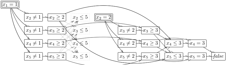
Example 2 Consider a problem P ≡ (C,D) where C ≡ {∑5i=1 xi ≤ 12, alldiff ({x1, x2, x3, x4, x5})} and D(xi) = {1 .. 8}, 1 ≤ i ≤ 5. If the search chooses x1 = 1 we arrive at subproblem P1 = (C ∪ {x1 = 1}, D). Then, the alldiff constraint determines that x2 ̸= 1 from set of literals {x1 = 1} (i.e., with explanation {x1 = 1} → x2 ̸= 1), and similarly for x3, x4 and x5. This builds the second column of the implication graph in Figure 1. Then, the relation between literals for x2 determine that x2 ≥ 2 from {x2 ̸= 1} and similarly for the literal relationships of x3, x4, and x5, building the third column. The sum constraint determines that the upper bound of each of x2, x3, x4 and x5 is 5 from the lower bounds in the third column, thus building the fourth column. The new domain is D′ (x1) = {1}, D′ (xi) = {2 .. 5}, 2 ≤ i ≤ 5. If the search now chooses x2 = 2, we arrive at subproblem P2 = (C ∪ {x1 = 1, x2 = 2},D′ ). Then, the alldiff constraint determines x3 ̸= 2, x4 ̸= 2, and x5 ̸= 2 (the 6th column) from {x2 = 2}. The literal relationships determine that x3 ≥ 3 from {x3 ≥ 2, x3 ̸= 2}, similarly for x4 and x5. The sum constraint determines that x4 ≤ 3 from {x2 = 2, x3 ≥ 3, x5 ≥ 3}, similarly for x5 ≤ 3. Then, the literal relationships determine x4 = 3 from {x4 ≥ 3, x4 ≤ 3}, similarly for x5 = 3 and finally the alldiff constraint determines unsatisfiability of x4 = 3 and x5 = 3. ✷

A nogood N is a set of literals. A correct nogood N from problem P ≡ (C, D) is one where C ∧ D ⇒ ¬ ∧ℓ∈N ℓ, that is, in all solutions of P the conjunction of the literals in N is false. Given an implication graph, we determine a correct nogood that explains N → false by eliminating literals from N until only one literal at the current decision level remains. The result is the 1UIP (First Unique Implication Point) nogood, which the search records as a clausal propagator and backtracks to the decision level of the second latest literal in the nogood, where it applies the newly derived nogood.

Example 3 Continuing from Example 2 using the implication graph in Figure 1, we start with the explanation of failure {x4 = 3, x5 = 3} → false which gives us the initial nogood {x4 = 3, x5 = 3}. Since both literals were determined at the current decision level, we replace the last one x5 = 3 by the antecedents in its explanation {x5 ≥ 3, x5 ≤ 3} → x5 = 3 to obtain {x5 ≥ 3, x5 ≤ 3, x4 = 3}. We keep removing the last literal with the current decision level until only one literal remains at the current decision level. The resulting 1UIP nogood is {x2 ≥ 2, x3 ≥ 2, x4 ≥ 2, x5 ≥ 2, x2 = 2} which can be simplified to {x3 ≥ 2, x4 ≥ 2, x5 ≥ 2, x2 = 2}, since the last literal implies the first.

On backtracking to undo x2 = 2, the search arrives at subproblem P1 and immediately determines that x2 ̸= 2 using the new nogood. Importantly, if the search ever reaches a state where {x3 ≥ 2, x4 ≥ 2, x5 ≥ 2} holds, it will make the same inference. Indeed, if it reaches a point where {x2 = 2, x3 ≥ 2, x4 ≥ 2}, it will infer that x5 < 2. ✷

4 Symmetries and Nogoods

A symmetry of P ≡ (C,D) is a bijection ρ on the equality literals of P such that, for each valuation θ of P, ρ(θ) = {ρ(ℓ) | ℓ ∈ θ} is a solution of P iff θ is a solution of P . Variable symmetries, value symmetries and variable-value symmetries are all particular cases of symmetries.

Static Symmetry Breaking reduces the search by adding to C constraints that remove symmetric solutions. In particular, lexicographical constraints have been used to statically eliminate symmetries (see e.g.[Flener et al., 2002]) with excellent results. This is good news since static symmetry breaking is obviously compatible with lazy clause generation: we only require the new symmetry breaking constraints to have explaining propagators, which are then used just like other propagators. However, static symmetry breaking is not always the best option and, therefore, we are also interested in dynamic symmetry breaking.

Dynamic Symmetry Breaking techniques can be seen as pruning symmetric portions of the search space by using symmetric nogoods. In particular, if the search on subproblemP ′ fails, then choices(P ′ ) is a correct nogood of P (referred to as the choice nogood) and, therefore, any symmetric version of choices(P ′ ) is also a correct nogood of P. Note that the symmetric version of a nogood N with only equality literals is easy to define: ρ(N) = {ρ(ℓ) | ℓ ∈ N}.

Example 4 In problem P of Example 2, the variables {x1, x2, x3, x4, x5} are interchangeable (i.e., any two can be swapped). Since the subproblem P ′ with choices(P ′ ) = {x1 = 1, x2 = 2} fails, we know that {x1 = 1, x2 = 2} is a correct nogood for P. Clearly, any symmetric version, such as {x2 = 1, x1 = 2} or {x3 = 1, x5 = 2}, is also a correct nogood. ✷

Such nogoods can be used to prune search in two main ways. Symmetry breaking by dominance detection (SBDD) [Focacci and Milano, 2001; Fahle et al., 2001] keeps a store N of the non-subsumed choice nogoods derived during search so far. For each subproblem P ′ , it checks whether there exists N ∈ N and symmetry ρ, such that choices(P ′ ) ⇒ ρ(N). If such a pair exists it can immediately fail subproblem P ′ . Symmetry breaking during search (SBDS) [Gent and Smith, 2000], which is predated by the very similar [Backofen and Will, 1999], works as follows. Whenever a subproblem P ′ with choices(P ′ ) = {c1, c2, . . . , cn, cn+1} fails, SBDS backtracks to the parent subproblemP ′′ in level n and, for each symmetry ρ, it locally posts in P ′′ the conditional constraint (ρ(c1)∧. . .∧ρ(cn)) → ¬ρ(cn+1). Note that these constraints will only propagate when reaching a subproblem P ′′′ such that C ∪choices(P ′′′ ) entails the left hand side of the constraint. This will never happen if the symmetry is broken, i.e., if ∃ci s.t. ¬ρ(ci)

is entailed, and that is why SBDS ignores any symmetry ρ which is known to be broken at P ′′ . Still, SBDS can post too many local constraints when the number of symmetries is high. Thus, some incomplete methods ([Mears, 2010; Gent and Smith, 2000]) only post constraints that are known to immediately propagate.

We decided to integrate SBDS, rather than SBDD, with our lazy clause generation because SBDS is much closer to the lazy clause generation approach: they both compute and post nogoods. The main differences being that SBDS only computes decision nogoods and posts their symmetric versions.

5 Symmetries and Lazy Clause Generation

5.1 SBDS-choice

We can naively add SBDS to a lazy clause solver by simply using symmetric versions of the choice nogood at each node to prune off symmetric branches. Hence, we just re-implement standard SBDS in the lazy clause generation solver, but still gain the advantage of reduced search through the lazy clause generation nogoods.

5.2 SBDS-1UIP

Adapting SBDS to use 1UIP nogoods is simple: every time a 1UIP nogood {ℓ1, . . . , ℓn} → ℓn+1 is inferred for subproblem P ′ , upon backtracking to parent P ′′ and for each symmetry ρ, we post the symmetric nogood {ρ(ℓ1), . . . , ρ(ℓn)} → ¬ρ(ℓn+1), ignoring those ρ that are known to be broken at P ′′ . We can check this last condition during the construction of the symmetric nogood, as we produce the literals ρ(ℓ1), . . . , ρ(ℓn) one at a time. If at any point, one of ρ(ℓi) is false in P ′′ , we can immediately abort and move on to the next symmetry.

In contrast to SBDS-choice, in SBDS-1UIP we have to post the symmetric nogoods as global rather than local constraints. This is because in SBDS-choice, when you backtrack from parent P ′′ to grandparent P ′′′ , the choice nogood at P ′′′ subsumes that at P ′′ and, therefore, SBDS-choice will always post a set of symmetric nogoods that subsumes the symmetric nogoods posted below that point. In contrast, there is no guarantee that the 1UIP nogood at P ′′′ subsumes the one at P ′′ (and in general it does not). This means that many nogoods can be are added at each node. However, this is not a big problem. Nogood propagation in LCG solvers is very fast since they use the same efficient handling of clauses used in SAT solvers. In addition, activity counts are kept for each nogood and inactive nogoods are periodically pruned just as in SAT solvers.

Example 5 Consider the problem of Example 2. On backtracking to P1 we infer the nogood {x3 ≥ 2, x4 ≥ 2, x5 ≥ 2} → x2 ̸= 2. With this we not only infer x2 ̸= 2 but also the symmetric inferences x3 ̸= 2 (from {x2 ≥ 2, x4 ≥ 2, x5 ≥ 2}), x4 ̸= 2 and x5 ̸= 2. At this point, a domain consistent alldiff will determine failure and generate ∅ → x1 ̸= 1, which does not subsume the previously generated nogood. ✷

We show that SBDS-1UIP exploits strictly more symmetries than SBDS-choice if the asserting literals in the nogoods are the same, and propagation has the following property:

Definition 1 A set of propagators for problem P has global symmetric monotonicity iff, for any explanation {c1, . . . , cn} → ℓ produced and any symmetry ρ of P , whenever ρ(c1), . . . , ρ(cn) are entailed, ρ(ℓ) is also entailed. ✷

A sufficient condition for global symmetric monotonicity is the following: all propagators are monotonic, and all symmetries are propagator symmetric (i.e., the symmetry maps propagators to propagators). Global symmetric monotonicity is therefore very common, as most propagators are monotonic, and the vast majority of symmetries that are usually exploited are propagator symmetric.

Theorem 1 Suppose global symmetric monotonicity holds, and we derive choice nogood {c1, . . . , cn} → ¬cn+1, and 1UIP nogood {ℓ1, . . . , ℓm} → ¬cn+1 from the same conflict. If {ρ(c1), . . . , ρ(cn)} → ¬ρ(cn+1) propagates then so does {ρ(ℓ1), . . . , ρ(ℓm)} → ¬ρ(cn+1). ✷

The theorem shows that the symmetric 1UIP nogood subsumes the symmetric choice nogood, since it will always produce any implication that the symmetric choice nogood can, but not vice versa. This means that SBDS-1UIP can exploit strictly more symmetry than SBDS-choice. This result is valid for both complete SBDS, as well as for incomplete SBDS methods which only post nogoods that will immediately produce an implication.

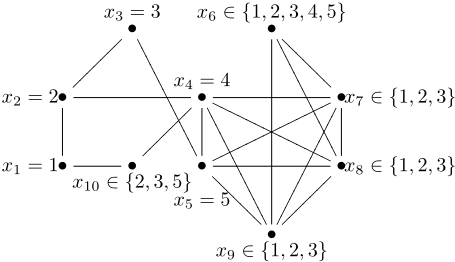
Example 6 Consider the graph colouring problem shown in Figure 2, where we are trying to colour the nodes with at most 5 colours (all of which are interchangeable). After making the decisions x1 = 1, x2 = 2, x3 = 3, x4 = 4, x5 = 5, we have domains as shown in Figure 2. Suppose we label x6 = 1 next. Then propagation gives x7 ∈ {2, 3}, x8 ∈ {2, 3}, x9 ∈ {2, 3}. Now, suppose we try x7 = 2. This forces x8 = 3, x9 = 3, which conflicts. The 1UIP nogood from this conflict is {x8 ̸= 1, x8 ̸= 4, x8 ̸= 5, x9 ̸= 1, x9 ̸= 4, x9 ̸= 5} → x7 ̸= 2. After propagating this nogood, we have x7 = 3, which after further propagation, once again conflicts. At this point, we backtrack to before x6 is labelled and derive the nogood {x7 ̸= 4, x7 ̸= 5, x8 ̸= 4, x8 ̸= 5, x9 ̸= 4, x9 ̸= 5} → x6 ̸= 1.

Now, let us examine what SBDS-1UIP can do at this point. It is clear that if we apply the value symmetries: 1 is symmetric to 2 (≪1≫⇆≪2≫), or ≪1≫⇆≪3≫ to this nogood; the LHS remains unchanged while the RHS changes. Therefore, we can post these two symmetric nogoods and immediately get the inferences x6 ̸= 2 and x6 ̸= 3. On the other hand, SBDS-choice cannot do anything. The choice nogood is {x1 = 1, x2 = 2, x3 = 3, x4 = 4, x5 = 5} → x6 ̸= 1, and it is easy to see that no matter which value symmetry we use on it, the LHS will have a set of literals incompatible with the current set of decisions and, thus, cannot imply the RHS. ✷

The kind of redundancy we exploit here certainly arises from symmetry. However, it is extremely difficult to exploit. Roughly speaking, we can say that we are exploiting the symmetry that exists in the sub-component of a subproblem which is the actual cause of failure. In this case, they are the variables x6, x7, x8, x9, their current domains in the subproblem, and the constraints linking them. Even conditional symmetry breaking constraints are powerless to exploit such symmetries, as the subproblem shown in Figure 2 does not have the value symmetries ≪1≫⇆≪2≫ or ≪1≫⇆≪3≫ due to the existence of x10. It is only because a lazy clause solver gives us such precise information about which variables are involved in failures that we can exploit this kind of redundancy. While the above example might seem contrived, our experiments in Section 7 show that these kinds of redundancies do occur in practice and can yield big speedups.

6 Symmetries on 1UIP nogoods

While SBDS-1UIP is much more powerful than SBDSchoice, having to manipulate 1UIP nogoods has its problems: unlike the choice nogoods which usually only involve equality literals on search variables, 1UIP nogoods can contain virtually any literal in the problem, including disequality and inequality literals, and also literals with intermediate variables.

6.1 Disequality and Inequality Literals

One of the strengths of lazy clause generation is the use of equality, disequality and inequality literals in explanations and nogoods. This can make explanations shorter and is essential for explaining bounds propagation. Thus, we need to extend symmetries to work with all literals.

Extending symmetry ρ to handle disequalities is straightforward: if ρ(x = d) ≡ x′ = d′ , then ρ(x ̸= d) ≡ x′ ̸= d′ . Extending ρ to handle inequalities is also straightforward for a variable symmetry σ: if ρ(x = d) ≡ x′ = d, then ρ(x ≤ d) ≡ x′ ≤ d and ρ(x ≥ d) ≡ x′ ≥ d. However, it is not clear how to extend value and variable-value symmetries. Thus, before we apply such symmetries we transform nogoods by replacing any of their inequality literals by an equivalent set (conjunction) of disequality literals (e.g. x ≤ 3 is replaced by x ̸= 4, x ̸= 5, x ̸= 6 assuming an initial domain [1..6]). Note that, while this transformation is theoretically correct, it may create very unwieldy nogoods.

6.2 Intermediate variables

An important problem for combining dynamic symmetry breaking and lazy clause generation is the fact that intermediate variables may be introduced in the course of converting a high level model to the low level variables and constraints implemented by the solver. If the symmetry declaration was made in the high level model, it may not specify how literals on the intermediate variables map to each other. Thus, we must extend symmetries to include such literals.

In some cases intermediate variables are idempotent under the symmetries, i.e., for each symmetry ρ of P, we can extend ρ to ρ′ where ρ′ (ℓ) = ρ(ℓ) if vars(ℓ) ⊆ vars(C) and ρ′ (ℓ) = ℓ otherwise. The extended ρ′ is a symmetry of P with intermediate variables. We can imagine automating the proof of idempotence of intermediate variables under symmetries.

Example 7 Consider a model for concert hall scheduling. Every two values in {1 .. k} for the k identical concert halls are symmetrical (can be swapped). The model includes the constraint xi = k + 1 ∨ xj = k + 1 ∨ xi ̸= xj for all concerts i and j which overlap in time. In a flattened form we introduce new Boolean variables diff i,j ⇔ xi ̸= xj and notoni ⇔ xi = k + 1 (indicating concert i is not scheduled) to represent disjuncts of this constraint. Since each introduced notoni and diff i,j variable is idempotent under the value symmetries, any symmetry ρ on the original variables can be trivially extended. ✷

Sometimes we can manually extend our symmetry declarations to take into account the intermediate variables. Other times it is not easy to see how to extend symmetries to all intermediate variables, and indeed quite often intermediate variables are introduced far below the modelling level. In order to handle these cases we modify learning as follows. We extend the model to explicitly mark which literals are allowed to appear in nogoods. We then modify the learning process to always explain unmarked literals. There is a requirement that all literals generated by search are allowed to appear in nogoods. This ensures that the process always terminates and always generates an asserting nogood.

In summary the SBDS-1UIP method is as follows:

• Identify any intermediate variables introduced by flattening or by the solver
• Attempt to extend any symmetry declarations to include these variables
• If the last step is not possible, make a declaration to the solver that literals on these intermediate variables are not allowed to be used in nogoods
• When a 1UIP nogood is derived by standard conflict analysis, examine all symmetric versions of it and post any that can immediately propagate
• Handle these extra nogoods in the same way as normal nogoods, i.e. post as clausal propagators, periodically prune inactive ones

7 Experiments

We now provide experimental evidence that symmetry breaking with 1UIP nogoods is superior to using only choice nogoods and that exploiting the redundancies such as those in Example 6 gives improved performance. The two problem we examine are the Concert Hall Scheduling problem (which has value symmetries as explained in Example 7 and variable symmetries for identical concerts) and the Graph Colouring problem (which has value symmetry on colors, and variable symmetries for nodes with the same set of neighbours). We take the benchmarks originally used by the authors of [Law et al., 2007]. The benchmarks are available at http://www. cmears.id.au/symmetry/symcache.tar.gz.

We implemented SBDS in CHUFFED, which is a state of the art lazy clause solver. We run CHUFFED with three different versions of SBDS: choice, where we use symmetric versions of choice nogoods, 1UIP, where we use symmetric versions of 1UIP nogoods, and crippled, where we use symmetric versions of 1UIP nogoods, but only those nogoods derived from symmetries where choice could also exploit the symmetry. We compare against CHUFFED with no symmetry breaking (none) and with standard lexicographical symmetry breaking constraints (static). Finally, we compare against an implementation of SBDS in [Mears, 2010] called Lightweight Dynamic Symmetry Breaking (LDSB), which is implemented in Eclipse and is the fastest dynamic symmetry breaking implementation on the two problems we examine, beating GAP-SBDS and GAP-SBDD by significant margins.

All versions of CHUFFED were run on Xeon Pro 2.4GHz processors. The results for LDSB were run on a Core i7 920 2.67 GHz processor. Times displayed are the average run times for all instances of each size. Instances which timeout (at 600s) are counted as 600 seconds.

The results are shown in Tables 1 and 2. Note that the Eclipse solver reports nodes, the number of internal nodes, but since the tree is binary and there are not many solutions this is comparable with failure counts. Eclipse LDSB fails to solve many instances before timeout, and choice fails to solve a few instances. 1UIP, crippled and static all solve every instance in the benchmarks. In fact, this set of instances, which is of an appropriate size for normal CP solvers, is a bit too easy for lazy clause solvers such as CHUFFED, as is apparent from the run times.

Comparison between choice and 1UIP shows that SBDS1UIP is superior to SBDS-choice. Comparison between crippled and 1UIP shows that the additional symmetries that we can only exploit with SBDS-1UIP indeed gives us reduced search and additional speedup. Comparison with static shows that dynamic symmetry breaking can be superior to static symmetry breaking on appropriate problems. The comparison with LDSB shows that lazy clause with symmetry breaking explores orders of magnitude less nodes.