
Large Linear Classification When Data Cannot Fit in Memory
Proceedings of the Twenty-Second International Joint Conference on Artificial Intelligence. Pages 2777-2781.
https://doi.org/10.5591/978-1-57735-516-8/IJCAI11-462
© 2011 International Joint Conferences on Artificial Intelligence
Abstract
Linear classification is a useful tool for dealing with large-scale data in applications such as document classification and natural language processing. Recent developments of linear classification have shown that the training process can be efficiently conducted. However, when the data size exceeds the memory capacity, most training methods suffer from very slow convergence due to the severe disk swapping. Although some methods have attempted to handle such a situation, they are usually too complicated to support some important functions such as parameter selection. In this paper, we introduce a block minimization framework for data larger than memory. Under the framework, a solver splits data into blocks and stores them into separate files. Then, at each time, the solver trains a data block loaded from disk. Although the framework is simple, the experimental results show that it effectively handles a data set 20 times larger than the memory capacity.
- [Bertsekas, 1999] Dimitri P. Bertsekas. Nonlinear Program- ming. Athena Scientific, Belmont, MA 02178-9998, sec- ond edition, 1999.
- yahoo-korea: Function value reduction. ((b)) webspam: Function value reduction. ((c)) epsilon: Function value reduction.
- d)) webspam: Testing performance. ((e)) yahoo-korea: Testing performance. ((f)) epsilon: Testing performance. Figure 2: The relative function value difference to the minimum (top row) and the accuracy difference to the best testing accuracy (bottom row). Time (in seconds) is log scaled. The blue dotted vertical line indicates time spent by Algorithms 1- based methods for the initial split of data to blocks. Note that in Figure 2(f), the curve of BLOCK-L-D is not connected, where the missing point corresponds to the best accuracy. [Bottou, 2007]
- Leon Bottou. Stochastic gradient de- scent examples, 2007. http://leon.bottou.org/ projects/sgd. Link
- [Breiman, 1996] Leo Breiman. Bagging predictors. Machine Learning, 24(2):123-140, August 1996.
- [Chang and Lin, 2001] Chih-Chung Chang and Chih-Jen Lin. LIBSVM: a library for support vector machines, 2001. Software available at http://www.csie.ntu. edu.tw/˜cjlin/libsvm. Link
- [Chang et al., 2007] Edward Chang, Kaihua Zhu, Hao Wang, Hingjie Bai, Jian Li, Zhihuan Qiu, and Hang Cui. Parallelizing support vector machines on distributed com- puters. In NIPS 21, 2007.
- [Fan et al., 2008] Rong-En Fan, Kai-Wei Chang, Cho-Jui Hsieh, Xiang-Rui Wang, and Chih-Jen Lin. LIBLINEAR: A library for large linear classification. JMLR, 9:1871- 1874, 2008.
- [Hsieh et al., 2008] C.-J. Hsieh, K.-W. Chang, C.-J. Lin, S. S. Keerthi, and S. Sundararajan. A dual coordinate de- scent method for large-scale linear SVM. In ICML, 2008.
- [Joachims, 1998] Thorsten Joachims. Making large-scale SVM learning practical. In Advances in Kernel Methods - Support Vector Learning. MIT Press, 1998.
- [Joachims, 2006] T. Joachims. Training linear SVMs in lin- ear time. In ACM KDD, 2006. [Memisevic, 2006] Roland Memisevic. Dual optimization of conditional probability models. Technical report, Depart- ment of Computer Science, University of Toronto, 2006.
- [Morse, 2005] Kingsley G. Morse, Jr. Compression tools compared. Linux Journal, 2005.
- [Pérez-Cruz et al., 2004] Fernando Pérez-Cruz, Aníbal R. Figueiras-Vidal, and Antonio Artés-Rodríguez. Double chunking for solving SVMs for very large datasets. In Pro- ceedings of Learning 2004, Spain, 2004.
- [Shalev-Shwartz et al., 2007] S. Shalev-Shwartz, Y. Singer, and N. Srebro. Pegasos: primal estimated sub-gradient solver for SVM. In ICML, 2007.
- [Yu et al., 2010] Hsiang-Fu Yu, Cho-Jui Hsieh, Kai-Wei Chang, and Chih-Jen Lin. Large linear classification when data cannot fit in memory. In ACM KDD, 2010.
- [Zhu et al., 2009] Zeyuan A. Zhu, Weizhu Chen, Gang Wang, Chenguang Zhu, and Zheng Chen. P-packSVM: Parallel primal gradient descent kernel SVM. In ICDM, 2009.
- [Zinkevich et al., 2010] Martin Zinkevich, Markus Weimer, Alex Smola, and Lihong Li. Parallelized stochastic gradi- ent descent. In NIPS 23, pages 2595-2603. 2010.
References were extracted automatically from the PDF and may contain errors.
Full text extracted automatically from the PDF; figures, tables and equations may differ. The PDF is the version of record.
1 Introduction
As the availability of annotated data increases steadily, data size becomes larger and larger. For example, it takes around 40 MB main memory to train the largest data in a data mining challenge kddcup 2004, and 1.6GB in kddcup 2009. In kddcup 2010, the size becomes about 10GB. 1 In a visual recognition challenge ImageNet 2 in 2010, the winner reports that their method involves training a data set in hundreds of gigabytes.
Linear classification is a promising tool for learning on huge data with large numbers of instances as well as features. Recent developments on linear classification (e.g., [Joachims, 2006; Shalev-Shwartz et al., 2007; Bottou, 2007; Hsieh et al., 2008]) have shown that training one million instances takes only a few seconds if data is already loaded in the memory. Therefore, some have said that linear classification is essentially a solved problem when the memory is et al., 2010] for large linear classification when data is stored in disk. BM splits the entire data into several subsets. Then, it iteratively loads and trains a subset of data. The method enjoys the following properties:
1 Of course the data size depends on the features extracted from the data.
2 http://www.image-net.org
- BM is simple and can easily support functions such as multi-class learning and parameter selection.
- BM is proven to converge to a global minimum of a function defined on the entire data, even though it updates the model on a local subset of data at each time.
- In practice, BM deals with memory problem effectively. We show in Section 6 that BM handles a data which is 20 times larger than the memory capacity and BM is more efficient than other methods.
This paper is organized as follows. In Section 2, we consider SVM as our linear classifier and introduce a block minimization framework. Two implementations of the framework for primal and dual SVM problems are respectively in Sections 3 and 4. Section 5 reviews some related approaches for data larger than memory. We show experiments in Section 6 and give conclusions in Section 7.
A detailed version of this paper is in [Yu et al., 2010].
2 BlockMinimization for Linear SVMs
Given a data set {(xi, yi)}li=1 , xi ∈ Rn, yi ∈ {-1, +1}, linear classifiers solve the following unconstrained optimization problem:
where C > 0 is a penalty parameter, 1/2wT w is the regularization term, and ξ (w; xi, yi) is the loss function. Three common loss functions are
Logistic Regression : log(1 + e-yiwT xi ).
After solving (2), we get the model w. The prediction can then be done by computing wT x for any incoming instance x. Problem (2) is often referred to as the primal form of classification problems. One may instead solve its dual problem. Here we only show the dual form of L1-SVM 3 :
where e = [1, . . . , 1]T and Qij = yiyjxTi xj. After obtaining the optimal solution α∗ for (3), the model w can then be computed by
Most linear SVM solvers assume data is stored in the memory so that the data can be randomly accessed. Therefore, Algorithm 1 A block minimization framework for linear SVM
3 The dual forms for L2-SVM and LR are similar, see [Hsieh et al., 2008] and [Yu et al., 2010]
- Split {1, . . . , l} to B1, . . . ,Bm and store data into m files accordingly.
- Set initial α or w
- For k = 1, 2, . . . (outer iteration)
For j = 1, . . . ,m (inner iteration)
- Read xr, ∀r ∈ Bj from disk
- Conduct operations on {xr | r ∈ Bj}
- Update α or w
when data cannot fit in memory, such methods suffer from disk swapping. With limited memory, a viable method must satisfy the following conditions:
- Each optimization step reads a continuous chunk of training data.
- The optimization procedure converges toward the optimum even though each step trains only a subset of data.
- The number of optimization steps (iterations) need be small. Otherwise, the amount of disk access will be huge.
Obtaining a method having all these properties is not easy.
As entire data cannot fit in memory, we consider loading a block of data at a time. In the following, we show that with a careful design, a block minimization can fully utilize the data in the memory before loading another data block from the disk.
Let {B1, . . . ,Bm} be a partition of all data indices {1, . . . , l}. We adjust the block size such that instances associated with Bj can fit in memory. These m blocks, stored as m files, are loaded when needed. Then, at each step, we conduct some operations using one data block, and update w or α according to if the primal or the dual problem is considered. The block minimization framework is summarized in Algorithm 1. We refer to the step of working on a single block as an inner iteration, while the m steps of going over all blocks as an outer iteration. Algorithm 1 can be applied on both the primal form (2) and the dual form (3). We show two implementations in Sections 3 and 4, respectively.
Block minimization is a classical technique in optimization (e.g., [Bertsekas, 1999, Chapter 2.7]). Many studies have applied block minimization to train SVM or other machine learning problems, but we might be the first to consider it in the disk level.
Assume B1, . . . ,Bm have a similar size |B| = l/m. The time cost of Algorithm 1 is
where
- Tm(|B|) is the cost of operations at each inner iteration;
- Td(|B|) is the cost to read a block of data from disk.
These two terms respectively correspond to the two parts in (1) for modeling the training time.
Regarding the block size |B|, if data are stored in memory in advance, Td(|B|) = 0. For Tm(|B|), people observe that if |B| linearly increases, then
Tm(|B|) is generally more than linear to |B|, so Tm(|B|) × l/|B| is increasing along with |B|. In contrast, the #outeriters may not decrease as quick. Therefore, nearly all existing SVM packages use a small |B|. For example, |B| = 2 in LIBSVM [Chang and Lin, 2001] and 10 in SVMlight [Joachims, 1998].
However, when data cannot be stored in the memory, Td(|B|) > 0 and the situation is different. At each outer iteration, the cost is
The second term is for loading l instances from disk. As reading each data block takes some initial time, a smaller number of blocks reduces the cost. Hence the second term in (4) is a decreasing function of |B|. While the first term is increasing following the earlier discussion, as reading data from the disk is slow, the second term is likely to dominate. Therefore, contrary to existing SVM software, in our case the block size should not be too small.
Moreover, since the loading time Td(B) is proportional to the size of data, we can reduce the size of each data blocks by storing a compressed file in the disk. However, we then need some additional time to decompress the data when each block is loaded. The balance between compression speed and ratio has been well studied in the area of backup and networking tools [Morse, 2005]. We choose a widely used compression library zlib for our implementation. 4 The detailed discussion of implementation issues can be found in [Yu et al., 2010].
3 Solving Dual SVM for Each Block
A nice property of the SVM dual problem (3) is that each variable corresponds to a training instance. Thus we can easily devise an implementation of Algorithm 1 by updating a block of variables at a time. Assume ¯Bj = {1, . . . , l}\Bj, at each inner iteration we solve the following sub-problem.
That is, we change αBj using the solution of (5), while fix α¯Bj . Then Algorithm 1 reduces to the standard block minimization procedure, so the convergence to the optimal function value of (3) holds [Bertsekas, 1999, Proposition 2.7.1].
We must ensure that at each inner iteration, only one block of data is needed. With the constraint d ¯Bj = 0 in (5),
4 http://www.zlib.net
Algorithm 2 An implementation of Algorithm 1 for solving dual SVM
We only show details of steps 3.2 and 3.3:
- Exactly or approximately solve the sub-problem (5) to obtain d∗Bj
- αBj ←αBj + d∗Bj
Update w by (8)
where QBj,: is a sub-matrix of Q including elements Qri, r ∈ Bj, i = 1, . . . , l. Clearly, QBj,: in (6) involves all training data, a situation violating the requirement in Algorithm 1. Fortunately, by maintaining
we have
Therefore, if w is available in memory, only instances associated with the block Bj are needed. To maintain w, if d∗Bj is an optimal solution of (5), we consider (7) and use
This operation again needs only the block Bj . The procedure is summarized in Algorithm 2.
For solving the sub-problem (5), as all the information is available in the memory, any bound-constrained optimization method can be applied. We consider LIBLINEAR [Fan et al., 2008], which implements a coordinate descent method (i.e., block minimization with a single element in each block). Then, Algorithm 2 becomes a two-level block minimization method. The two-level setting had been used for SVM or other applications (e.g., [Memisevic, 2006; P´erez-Cruz et al., 2004]), but ours might be the first to associate the inner level with memory and the outer level with disk.
Under this framework, we can either accurately or loosely solves the sub-problem of block Bj :
- Loosely solving the sub-problem: A simple setting is to go through all variables in Bj a fixed number of times. A small number of passes over Bj means to loosely solve the sub-problem (5). While the cost per block is cheaper, the number of outer iterations may be large.
- Accurately solving the sub-problem: Alternately, we can accurately solve the sub-problem. The cost per inner iteration is higher, but the number of outer iterations may be reduced. As an upper bound on the number of iterations does not reveal how accurate the solution is, most optimization software consider the gradient information.
When the sub-problem solvers satisfy certain conditions, Algorithm 1 globally converges to an optimal solution α∗ with linear rate. That is, there are 0 < μ < 1 and an iteration k0 such that
In [Yu et al., 2010], we prove that the linear convergence holds when the sub-problems are solved with a fixed number of passes or the gradient stopping condition used in LIBLINEAR.
Algorithm 3 An implementation of Algorithm 1 for solving primal SVM. Each inner iteration is by Pegasos
- Split {1, . . . , l} to B1, . . . ,Bm and store data into m files accordingly.
- t = 0 and initial w = 0.
- For k
- = 1, 2, . . .
For j = 1, . . . ,m
- Find a partition of Bj: B1 j , . . . ,B ¯ r j .
- For r = 1, . . . , ¯ r
- Use Br j as B to conduct the update (9)-(11).
- t ← t + 1
4 Solving Primal SVM for Each Block
Instead of solving the dual problem, in this section we check if the framework in Algorithm 1 can be used to solve the primal problem. Since the primal variable w does not correspond to data instances, we cannot use a standard block minimization setting to have a sub-problem like (5). In contrast, existing stochastic gradient descent methods possess a nice property that at each step only certain data are used. In this section, we study how Pegasos [Shalev-Shwartz et al., 2007] can by used for implementing an Algorithm 1.
Pegasos considers a scaled form of the primal SVM problem:
At the tth update, Pegasos chooses a block of data B and updates the primal variable w by a stochastic gradient descent step:
where ηt = lC/t is the learning rate, ∇t is the sub-gradient
and B+ ≡ {i ∈ B | yiwT xi < 1}. Then Pegasos obtains w by scaling ¯w:
Clearly we can directly consider Bj in Algorithm 1 as the set B in the above update. Alternatively, we can conduct several Pegasos updates on a partition of Bj . Algorithm 3 gives details of the procedure.
In this paper, we consider splitting Bj to |Bj| sets, where each one contains an element in Bj. We then conduct |Bj| Pegasos updates in Step 3.2 of Algorithm 3. The comparison for other settings can be found in [Yu et al., 2010].
5 Related Approaches for Large-scale Data
In this section, we discuss related methods for training linear model when data is larger than the memory size. Existing methods include:
Parallelizing batch learners Some approaches (e.g., [Chang et al., 2007; Zhu et al., 2009]) consider solving huge data set in distributed systems by a parallel scheme. Although such approaches can scale up to large data, they are usually complicated and induce expensive communication/synchronization overheads. Moreover, distributed systems may not be easily accessed by a ordinary user.
Sub-sampling In many cases, sub-sampling training data does not downgrade the prediction accuracy much. Therefore, by randomly drawing some training samples and storing them in memory, we can employ standard training techniques. This approach usually works when the data quality is good. However, in some situations, dealing with huge data may still be necessary. In Section 6.2, we show the relationship between testing performance and sub-sampled size.
Bagging Bagging [Breiman, 1996] averages models trained on subsets of data. A bagging method randomly draws m subsets of samples from the entire data set, and then trains m models w1, . . . ,wm, separately. The final model is obtained by averaging these m models. Although a bagging method can be easily parallelized and sometimes achieves an accurate model [Zinkevich et al., 2010], it does not solve a specific formulation such as (2).
Online Learning Online learners assume each time one data point is randomly drawn from a probability distribution. According to this data point, they then update the model w to minimize the expected loss. As the update rule is simple and only depends on one data point, online methods are suitable for handling the situation that data exceeds the memory size. For example, a recent software Vowpal Wabbit 5 handles large data by cyclically loading each data instance into memory and conducting an online sub-gradient descent update. It also supports the setting to pass over data several times. During the first pass, it saves the data points into a compressed cache file to speed up the reading time for the following passes. This is similar to our data compression strategy mentioned in Section 2. Note that Vowpal Wabbit solves a non-regularized problem, which is different from (2).
6 Experiments
In this section, we first show that sub-sampling data to fit in memory may downgrade the accuracy on the data we considered. Then, we demonstrate that block minimization methods are effective and efficient for training a data set larger than memory capacity. A detailed comparison demonstrating the influence of various settings under the block minimization framework can be founded in [Yu et al., 2010].
6.1 Data and Experimental Environment
We consider two document data sets yahoo-korea 6 andwebspam, and an artificial data epsilon. 7 Table 1 summarizes the data statistics.
We randomly split the data such that 4/5 for training and 1/5 for testing. All feature vectors are instance-wisely scaled to unit-length (i.e., ‖xi‖ = 1, ∀i). For epsilon, each feature of is normalized to have mean zero and variance one, and the testing set is modified according to the same scaling factors. This feature-wise scaling is conducted before the instancewise scaling. The value C in (2) is set to one.
5 The software is available at http://hunch.net/˜vw/.
6 This data set is not publicly available
7 webspam and epsilon can be downloaded at http:// largescale.first.fraunhofer.de
| Data set | l | n | #nonzeros | Memory (Bytes) |
|---|---|---|---|---|
| yahoo-korea | 460,554 | 3,052,939 | 156,436,656 | 2,502,986,496 |
| webspam | 350,000 | 16,609,143 | 1,304,697,446 | 20,875,159,136 |
| epsilon | 500,000 | 2,000 | 1,000,000,000 | 16,000,000,000 |
We conduct experiments on a 64-bit machine with 1GB RAM. Due to the space consumed by the operating system, the real memory capacity we can use is 895MB. Note that the size of the largest data, webspam, is 20 times larger than the size of memory.
6.2 Data Sub-sampling
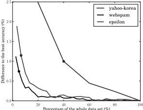
In some applications, training on a subset of data achieves similar performance as on the entire data. However, in other cases, sub-sampling may harm the testing performance. To investigate the performance of sub-sampling, we show the testing performance along data size in Figure 3. Result indicates that using a subset may not be enough to obtain a reasonable model in our case.
6.3 Training Time and Testing Accuracy
Next, we investigate the performance of block minimization methods. We compare the following methods:
- BM-LIBLINEAR: Algorithm 2 with LIBLINEAR to solve each sub-problem. For each sub-problem, LIBLINEAR goes through the data block 10 rounds.
- BM-Pegasos: Algorithm 3 with ¯ r = |Bj|. That is, we apply |Bj| Pegasos updates, each of which uses an individual data instance.
- LIBLINEAR: The standard LIBLINEAR without any modification to handle the situation if data cannot fit in memory.
We make sure that no other jobs are running on the same machine and report wall clock time in all experiments. We include data loading time and, for Algorithm 1, the initial time to split and compress data into blocks. It takes around 228 seconds to split yahoo-korea, 1,594 seconds to split webspam and 1,237 seconds to split epsilon. For LIBLINEAR, the loading time for yahoo-korea is 103 seconds, 829 seconds for webspam and 560 seconds for epsilon.
We are interested in both how fast the methods reduce the objective function value (2) and how quickly the methods obtain a reasonable model. Therefore, we present the following results in Figure 2:
- Training time versus the relative difference to the optimum
where f P is the primal objective function in (2) andw∗ is the optimal solution. Since w∗ is not really available, we spend enough training time to get a reference solution.
- Training time versus the difference to the best testing accuracy
where acc(w) is the testing accuracy using the model w and acc∗ is the best testing accuracy among all methods.
Results show that LIBLINEAR suffers from slow training due to severe disk swapping. In contrast, since memory issues are carefully handled, BM-LIBLINEAR and BM-Pegasos are more efficient. Therefore, they obtain a reasonable solution much faster than LIBLINEAR. Further, BM-LIBLINEAR is slightly faster than BM-Pegasos. This is because BMPegasos only conducts a simple update on each instance, while BM-LIBLINEAR considers a data block at a time and utilizes the instances loaded in memory by multiple updates.
7 Conclusions
In summary, we introduce a block minimization framework for solving large linear classification problems when data cannot fit in memory. The approach is simple but effective. Experiments show that the block minimization methods can handle data 20 times larger than the memory size.
8 Acknowledgments
This work was supported in part by the National Science Council of Taiwan via the grant 98-2221-E-002-136-MY3.
@inproceedings{ijcai2011p462,
  title     = {Large Linear Classification When Data Cannot Fit in Memory},
  author    = {Yu, Hsiang-Fu and Hsieh, Cho-Jui and Chang, Kai-Wei and Lin, Chih-Jen},
  booktitle = {Proceedings of the Twenty-Second International Joint Conference on
               Artificial Intelligence, {IJCAI-11}},
  publisher = {AAAI Press/International Joint Conferences on Artificial Intelligence},
  editor    = {Toby Walsh},
  pages     = {2777--2781},
  year      = {2011},
  month     = {7},
  doi       = {10.5591/978-1-57735-516-8/IJCAI11-462},
  url       = {https://doi.org/10.5591/978-1-57735-516-8/IJCAI11-462},
}
TY - CPAPER TI - Large Linear Classification When Data Cannot Fit in Memory AU - Yu, Hsiang-Fu AU - Hsieh, Cho-Jui AU - Chang, Kai-Wei AU - Lin, Chih-Jen T2 - Proceedings of the Twenty-Second International Joint Conference on Artificial Intelligence, IJCAI-11 PB - AAAI Press/International Joint Conferences on Artificial Intelligence PY - 2011 SP - 2777 EP - 2781 DO - 10.5591/978-1-57735-516-8/IJCAI11-462 UR - https://doi.org/10.5591/978-1-57735-516-8/IJCAI11-462 ER -Copied
Machine-readable versions of this paper, for tools and AI agents:





