Flexible Tree Matching

1 Introduction

The problem of comparing trees arises naturally in diverse fields, including computational biology, compiler optimization, natural language processing, and computer vision [Bille, 2005]. The most common measure for gauging the similarity of two labeled trees is the edit distance metric, first introduced by Tai [1979], which computes the cost of transforming one tree into another through a sequence of elementary node operations such as insertion, deletion, and renaming. To calculate this distance, a minimum-cost correspondence is established between the nodes of the two trees in a process known as tree matching.

In the classical formulation, these correspondences are rigid: they are not allowed to violate ancestor-descendant relationships between nodes, nor the left-to-right order of a node's children. As a result of these structural requirements, the problem admits an efficient dynamic programming algorithm, and the optimal matching can be found in cubic time [Demaine et al., 2009]. If the ordering requirement is removed (but the ancestry requirement maintained), the edit distance computation becomes NP-complete [Zhang et al., 1992], and approximation algorithms are necessary [Shasha et al., 1994].

In some domains, the most appropriate matchings may not strictly preserve ancestry. For instance, while reparenting even a single node in a phylogenetic tree of bacteria would destroy its validity, the ancestry relationships in the Document Object Model tree of a Web page are much less prescriptive: moving a search bar from header to footer results in a different-but largely equivalent-page. This pattern follows for many other tree structures encountered in design and data management, in which hierarchy plays an important-but not definitive-role [Chawathe and Garcia-Molina, 1997].

We introduce flexible tree matching, which relaxes the requirement that the produced correspondence strictly preserve ancestry relationships. Instead, the algorithm provides a parameterized framework for controlling the relative import of labeling and hierarchy. Introduced in Kumar et al. [2011], the algorithm uses an edge-based cost model to match nodes with similar labels while simultaneously penalizing matchings which induce violations of the hierarchy or break up sibling groups. Determining the minimum edit distance between trees then reduces to finding a minimum-cost matching under this model.

We prove that flexible tree matching is NP-complete in the strong sense, and give a corresponding stochastic approximation algorithm. We also show how to learn the parameters of the model from a corpus of examples via standard structured prediction techniques, and summarize results from applying the method to automatic retargeting in Web design.

2 A Flexible Model for Tree Matching

A tree matching is an injective binary relation defined between two labeled trees T1 and T2. The relation can be viewed as a bipartite graph between the trees' nodes, with edges representing editing operations for transforming one tree into the other. Edges identifying nodes with dissimilar labels represent relabeling operations, while nodes which are not mapped correspond to insertions or deletions.

To differentiate between mappings, classical tree matching requires a model that defines the relabeling cost between nodes and the insertion/deletion cost for nodes which are not matched. Given such a model, the tree-matching problem is to find a lowest-cost mapping between trees which preserves ancestry: once two nodes m ∈ T1 and n ∈ T2 are matched, the descendants of m can only be matched to descendants of n, and vice versa.

Flexible matching relaxes this rigid ancestry requirement in favor of a tunable edge-based cost model. It forms a complete bipartite graph G between T1 ∪ {⊗1} and T2 ∪ {⊗2}, where ⊗1 and ⊗2 are auxiliary no-match nodes. Each edge in G is assigned a cost comprising three terms: a relabeling term cr, penalizing edges that connect nodes with different labels, an ancestry term ca, penalizing edges that violate ancestry relationships, and a sibling term cs, penalizing edges that break up sibling groups. The cost of an edge c(e) is the sum of these three terms, and the goal of flexible tree matching is to produce a set of edges M ⊂ G such that every node in T1 ∪ T2 is covered by precisely one edge and the total mapping cost c(M ) = 1 |T1|+|T2| ∑e∈M c(e) is minimized.

3 Exact Edge Costs

We define the cost of an edge e ∈ T1 × T2,

For edges in G connecting tree nodes to no-match nodes, we fix the cost c(e) = wn, where wn is a constant no-match penalty weight.

The relabeling term cr([m, n]) defines the cost of swapping the labels of nodes m and n. This function is domaindependent, and user-specified. If the labels are identical, cr([m, n]) = 0.

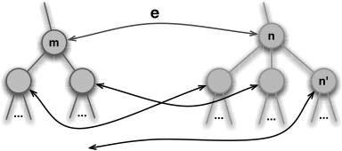
The ancestry cost ca(·) penalizes edges that violate ancestry relationships between the trees' nodes. Consider a node m ∈ T1, and let C(m) denote the children of m and M (m) denote the image of m in the matching. We define the ancestry-violating children of m, V (m), to be the set of m's children that map to nodes that are not M (m)'s children, i.e.,

and define V (n) symmetrically. Then, the ancestry cost for an edge is proportional to the number of ancestry violating children of its terminal nodes

where wa is a constant ancestry weight (see Figure 1).

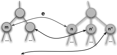
The sibling cost cs(·) penalizes edges that fail to preserve sibling relationships between trees. To calculate this term, we first define a few tree-related concepts. Let P (m) denote the parent of m. The sibling group of a node m comprises the children of its parent: S(m) = {C(P (m))}. Given a mapping M, the sibling-invariant subset of m, IM(m), is the set of nodes in m's sibling group that map to nodes in M (m)'s sibling group, i.e.,

the sibling-divergent subset of m, DM(m), is the set of nodes in m's sibling group that map to nodes in T2 not in M (m)'s sibling group, i.e.,

and the set of distinct sibling families that m's sibling group maps into is

We define all corresponding terms for n symmetrically, and then compute the total sibling cost

where ws is a constant sibling violation weight. The two ratios in the cost increase when siblings are broken up by the matching (i.e., their images have different parents), and decrease when siblings groups are maintained (see Figure 2). The FM(·) terms are included to guarantee that the total sibling penalty contributed by a tree is bounded by the number of nodes it contains.

4 Example Matchings

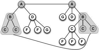
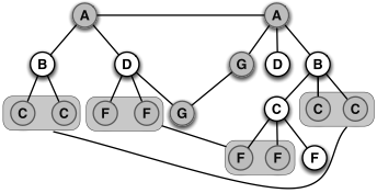
Figure 3 compares ordered, unordered, and flexible tree matching. In these examples, a simple relabeling function assigns a constant weight wr to all edges between tree nodes with differing labels. In ordered and unordered matching, the rigid preservation of ancestry leaves many nodes unmatched. In flexible matching, more common structure is preserved between the trees. By varying the terms in the cost model, different mappings can be achieved.

5 Flexible Tree Matching is NP-complete

We prove that flexible tree matching is strongly NPcomplete. We employ a simple version of the flexible cost Flexible Tree Matching wr = 1.0; wn = 1.0; wa = 0.5; ws = 0.5

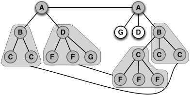
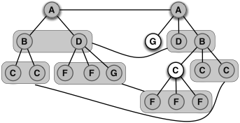
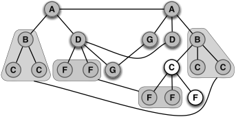
model from Section 4, where wr = 1, wn = 1, wa = 0, and ws = 1. That is, ancestry violations are forgiven but all relabelings, no-matches, and sibling violations are costly. Given this model and two labeled trees T1 and T2, we address the decision problem "Does there exist a zero-cost flexible mapping between the trees?"

This problem is in NP, since a proposed zero-cost mapping can be verified in polynomial time. To show that the problem is NP-hard, we formulate a polynomial-time reduction from 3-PARTITION [Garey and Johnson, 1975].

The 3-PARTITION problem is to decide whether a given multiset of integers can be partitioned into triples that all have the same sum. More formally, each instance is a finite set S of 3m integers, where each integer xi ∈ S satisfies K/4 < xi < K/2 for some bound K ∈ Z+ and ∑ xi = 3K. The question is to determine whether or not S can be partitioned into m disjoint sets U1, . . . ,Um, each with three elements, so that ∑u∈Ui u = K for every i ∈ {1, 2, . . . ,m}. This problem is NP-complete even when K is polynomial in m [Garey and Johnson, 1975].

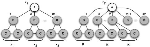
Given a 3-PARTITION instance, we construct trees T1 and T2 as in Figure 4. Each tree consists of three levels, and the nodes are labeled based on their level. T1 represents the set S, and contains 3m subtrees on the second level, with subtree i possessing xi leaf nodes. T2 contains m subtrees on the second level with K children each, and 2m more one-node subtrees. Since K is polynomial in m, this construction takes time polynomial in the size of the 3-PARTITION instance.

Under what circumstances can a zero-cost matching exist between these two trees? Since wn = 1, such a matching must map every node in T1 to some node in T2, and vice versa. Similarly, since wr = 1, the matching cannot identify nodes in different levels of the trees. Most importantly, since ws = 1, a zero-cost matching must preserve the 3m sibling groups of leaf nodes in T1: each of the m leaf node sibling groups in T2 must be matched to exactly three leaf node sibling groups in T1. Thus, a zero-cost matching exists only if the corresponding 3-PARTITION instance has a solution. Conversely, a solution to the 3-PARTITION instance indicates which leaf node sibling groups in T1 should be matched to a common leaf node sibling group in T2, naturally inducing a zero-cost matching.

This reduction implies that no polynomial-time (or even pseudopolynomial-time) algorithm can exist for flexible tree matching. For this reason, we propose a stochastic optimization algorithm for approximating the optimal matching, based on bounding the edge costs.

6 Bounding Edge Costs

While the cost model described in Section 3 balances labeling and structural constraints, it cannot be used to search for an optimal mapping M ⋆ directly. Although cr([m, n]) can be evaluated for an edge by inspecting m and n, ca(·) and cs(·) require information about the other edges in the mapping.

While we cannot precisely evaluate ca(·) and cs(·) a priori, we can compute bounds for them on a per-edge basis. Moreover, each time we accept an edge [m, n] into M, we can remove all the other edges incident on m and n from G. Each time we prune an edge in this way, the bounds for other nearby edges may be improved. Therefore, we employ a Monte Carlo algorithm to approximate M ⋆ , stochastically fixing an edge in G, pruning away the other edges incident on its nodes, and updating the bounds on those that remain.

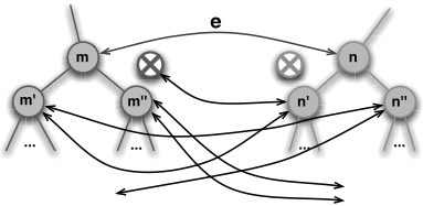
To bound the ancestry cost of an edge [m, n] ∈ G, we consider each child of m and n and answer two questions. First, is it impossible for this node to induce an ancestry violation? Second, is it unavoidable that this node will induce an ancestry violation? The answer to the first question informs the upper bound for ca(·); the answer to the second informs the lower.

A node m′ ∈ C(m) can induce an ancestry violation if there is some edge between it and a node in T2 \ (C(n) ∪ {⊗2}). Conversely, m′ is not guaranteed to induce an ancestry violation if some edge exists between it and a node in C(n) ∪ {⊗2} . Accordingly, we define indicator functions

Then, the upper and lower bounds for ca([m, n]; M ) are

and

Figure 5 illustrates the computation of these bounds. Pruning edges from G causes the upper bound for ca([m, n]; M ) to decrease, and the lower bound to increase.

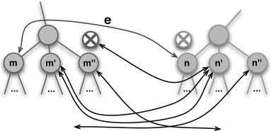
Similarly, we can bound cs([m, n]; M ) by bounding the number of divergent siblings, invariant siblings, and distinct families: |D(·)|, |I (·)|, and |F (·)|. Let ¯ S(m) = S(m) \ {m} and consider a node m′ ∈ ¯ S(m). It is possible that m′ is in DM(m) as long as some edge exists between it and a node in T2 \ ( ¯ S(n) ∪ {⊗2}). Conversely, m′ cannot be guaranteed to be in DM(m) as long as some edge exists between it and a node in ¯ S(n) ∪ {⊗2}. Then, we have

and

The bounds for |IM(m)| are similarly given by

and

For all nonzero sibling costs, the lower bound for |FM(m)| is 2 and the upper bound is LD(m, n) + 1. All remaining quantities are defined symmetrically. Then, upper and lower bounds for cs([m, n]; M ) are given by

and

Figure 6 illustrates the computations of the bounds for the sibling cost term.

With bounds for the ancestry and sibling terms in place, upper and lower bounds for the total edge cost are cU(e) = cr(e) + Ua(e) + Us(e) and cL(e) = cr(e) + La(e) + Ls(e).

7 Approximating the Optimal Mapping

To approximate the optimal mapping M ∗ , we use the Metropolis algorithm [Press et al., 2007]. We represent each matching as an ordered list of edges M, and define a Boltzmann-like objective function

where β is a constant. At each iteration of the algorithm, a newmapping ˆM is proposed, and becomes the new reference mapping with probability

The algorithm runs for N iterations, and the mapping with the lowest cost is returned.

To initialize M, the bipartite graph G is constructed and the edge bounds initialized. Then, the edges in G are traversed in order of increasing bound. Each edge is considered for assignment to M with some fixed probability γ, until an edge is chosen. If the candidate edge can be fixed and at least one complete matching still exists, it is appended to M, the other edges incident on its terminal nodes are pruned, and the bounds for the remaining edges in G are tightened.

To propose ˆM, we choose a random index j ∈ [1, |M|]. Then, we re-initialize G, and fix the first j edges in M. To produce the rest of the matching, we repeat the iterative edge selection process described above. In our implementation, we take γ = .7 and N = 100; β is chosen on a per-domain basis.

8 Learning Cost Models

While flexible tree matching can be used with any cost model comprising weights wr, wa, ws, and wn, it is often desirable to learn a model that will produce mappings with domaindependent characteristics. In particular, given a set of trees and exemplar matchings defined between them, we can use the generalized perceptron algorithm to learn weights under which the example matchings are minimal [Collins, 2002].

First, we reformulate the cost of a mapping c(M ) in terms of a weight vector w = 〈wr,wa,ws,wn〉. For each edge, we compute the difference between the real-valued labels of its terminal nodes and the exact ancestry and sibling costs, and concatenate these values along with a Boolean no-match indicator into a feature vector fe. The edge cost can then be computed as c(e) = wT fe. Given a mapping M, the algorithm assembles an aggregate feature vector FM = 1 |T1|+|T2| ∑e∈M fe to calculate the mapping cost c(M ) = wT FM .

In each training iteration, the perceptron randomly selects a pair of trees and an associated mapping M from the training set. Next, it computes a new mapping ˆM ≈ argminM wT i FM using the current cost model wi. For the first iteration, w0 = 0. Based on the resultant mapping, a new aggregate feature vector F ˆM is calculated, and the cost model is updated by wi+1 =wi +αi (F ˆM -FM ), where αi = 1/√i + 1 is the learning rate.

While the perceptron algorithm is only guaranteed to converge if the training set is linearly separable, in practice it produces good results for many diverse data sets [Collins, 2002]. Since the weights may oscillate during the final stages of the learning, the final cost model is produced by averaging over the last few iterations.

9 Case Study

Flexible tree matching was inspired by the goal of automatically retargeting Web pages [Kumar et al., 2011]. In this setting, the matching identifies semantically and structurally similar elements between pages to guide the transfer of content and design. We selected a corpus of 50 popular Web pages, and segmented the Document Object Model tree of each one to produce a hierarchy representative of its visual structure. In an online study, participants specified 117 matchings between 52 unique pairs of page trees. Then, using the method described in Section 8, we trained a cost model for flexible matching on this set.

In this domain, learning a consistent model for tree matching is complicated by the fact that humans do not produce identical mappings between pages. In our study, humans matchings are only 78.3% consistent, on average. Nonetheless, the flexible matching model is effective in this context, yielding matchings that average 68.7% similarity (and 77.7% under the nearest-neighbor metric) in a hold-out test.

Most Similar Most Dissimilar

Figure 9: The flexible treematching algorithm can be used to induce a distancemetric on the space of Web designs. Comparing the cost of matching the source page onto each of the targets can differentiate similar and dissimilar designs.

Once the cost model has been learned, the matchings it produces can be used to guide the transfer of content and design between pages (Figure 7-8). In addition, the algorithm provides an approximate distance metric on the space of page designs (Figure 9). See Kumar et al. [2011] for details.

10 Conclusion

This paper describes a tunable algorithm for flexible tree matching, with parameters that can be learned via structured prediction techniques. This algorithm may be useful for matching in many domains in which hierarchy is suggestive rather than definitive. We have demonstrated its efficacy on mapping between Web designs; future work could apply the technique to other design domains with hierarchical structure, such as 3D models or graphic design.