
Line Orthogonality in Adjacency Eigenspace with Application to Community Partition
Proceedings of the Twenty-Second International Joint Conference on Artificial Intelligence. Pages 2349-2353.
https://doi.org/10.5591/978-1-57735-516-8/IJCAI11-391
© 2011 International Joint Conferences on Artificial Intelligence
Abstract
Different from Laplacian or normal matrix, the properties of the adjacency eigenspace received much less attention. Recent work showed that nodes projected into the adjacency eigenspace exhibit an orthogonal line pattern and nodes from the same community locate along the same line. In this paper, we conduct theoretical studies based on graph perturbation to demonstrate why this line orthogonality property holds in the adjacency eigenspace and why it generally disappears in the Laplacian and normal eigenspaces. Using the orthogonality property in the adjacency eigenspace, we present a graph partition algorithm, AdjCluster, which first projects node coordinates to the unit sphere and then applies the classic k-means to find clusters. Empirical evaluations on synthetic data and real-world social networks validate our theoretical findings and show the effectiveness of our graph partition algorithm.
- [Chung et al., 2003] Fan Chung, Linyuan Lu, and Van Vu. Eigenvalues of random power law graphs. Annals of Com- binatorics, 7:21-33, 2003.
- [Davies and Bouldin, 1979] David Davies and Donald Bouldin. A cluster separation measure. IEEE Tran. on Pattern Analysis and Machine Intelligence, 1:224-227, 1979.
- [Golub and Van Loan, 1996] Gene H. Golub and Charles F. Van Loan. Matrix Computations. The Johns Hopkins Uni- versity Press, 1996.
- [Huang et al., 2008] Ling Huang, Donghui Yan, Michael I. Jordan, and Nina Taft. Spectral clustering with perturbed data. In NIPS, pages 705-712, 2008.
- [Miller and Teng, 1998] John R. Gilbert Gary L. Miller and Shang-Hua Teng. Geometric mesh partitioning: Imple- mentation and experiments. SIAM Journal on Scientific Computing, 19:2091-2110, 1998.
- [Prakash et al., 2010] B. Aditya Prakash, Ashwin Sridharan, Mukund Seshadri, Sridhar Machiraju, and Christos Falout- sos. Eigenspokes: Surprising patterns and scalable com- munity chipping in large graphs. In PAKDD, 2010.
- [Shi and Malik, 2000] Jianbo Shi and Jitendra Malik. Nor- malized cuts and image segmentation. IEEE Trans. on Pat- tern Analysis and Machine Intelligence, 22(8):888-905, 2000.
- [Stewart and Sun, 1990] G. W. Stewart and Ji-guang Sun. Matrix Perturbation Theory. Academic Press, 1990.
- [Viswanath et al., 2009] Bimal Viswanath, Alan Mislove, Meeyoung Cha, and Krishna P. Gummadi. On the Evo- lution of User Interaction in Facebook. In WOSN, 2009.
- [Wakita and Tsurumi, 2007] Ken Wakita and Toshiyuki Tsu- rumi. Finding community structure in mega-scale social networks: [extended abstract]. In WWW, pages 1275- 1276, 2007.
- [Ying and Wu, 2009] Xiaowei Ying and Xintao Wu. On ran- domness measures for social networks. In SDM, 2009.
References were extracted automatically from the PDF and may contain errors.
Full text extracted automatically from the PDF; figures, tables and equations may differ. The PDF is the version of record.
1 Introduction
Different from the Laplacian matrix or normal matrix, the properties of the adjacency eigenspace received much less attention except some recent work [Prakash et al., 2010; Ying and Wu, 2009]. It was shown by Prakash et al. [2010] that the singular vectors of mobile call graphs exhibit an EigenSpokes pattern wherein, when plotted against each other, they have clear, separate lines that neatly align along specific axes. The authors suggested that EigenSpokes are associated with the presence of a large number of tightlyknit communities embedded in very sparse graphs. Ying and Wu [2009] showed that node coordinates in the adjacency eigenspace of a graph with well structured communities form quasi-orthogonal lines (not necessarily axes aligned) and developed a framework to quantify importance (or non-randomness) of a node or a link by exploiting the line orthogonality property. However, no theoretical analysis was presented [Ying and Wu, 2009; Prakash et al., 2010] to demonstrate why and when this line orthogonality property holds.
In this paper, we conduct theoretical studies based on matrix perturbation theory. Our theoretical results demonstrate why the line orthogonality pattern exists in the adjacency eigenspace. Specifically we show that 1) spectral coordinates of nodes without direct links to other communities locate exactly on the orthogonal lines; 2) spectral coordinates of nodes with links to other communities deviate from lines; and 3) for a network with k communities there exist k orthogonal lines (and each community forms one line) in the spectral subspace formed by the first k eigenvectors of the adjacency matrix. We further give explicit formula (as well as its conditions) to quantify how much orthogonal lines rotate from the canonical axes and how far spectral coordinates of nodes with direct links to other communities deviate from the line of their own community. We also examine the spectral spaces of the Laplacian matrix and the normal matrix under the perturbation framework. Our findings show that the line orthogonality pattern in general does not hold in the Laplacian eigenspace or the normal eigenspace. We further provide theoretical explanations.
The discovered orthogonality property in the adjacency eigenspace has potential for a series of applications. In this paper, we present an effective graph partition algorithm, AdjCluster, which utilizes the line orthogonality property in the adjacency eigenspace. The idea is to project node coordinates (along the orthogonal lines) onto the unit sphere in the spectral space and then apply the classic k-means to find clusters. Our empirical evaluations on synthetic data and real-world social networks validate our theoretical findings and show the effectiveness of our graph partition algorithm .
2 Preliminaries
2.1 Notation
A network or graph G is a set of n nodes connected by a set of m links. The network considered here is binary, symmetric, connected, and without self-loops. It can be represented as the symmetric adjacency matrix An×n with aij = 1 if node i is connected to node j and aij = 0 otherwise. Let λi be the i-th largest eigenvalue of A and xi the corresponding eigenvector. xij denotes the j-th entry of xi. Formula (1) illustrates our notation. The eigenvector xi is represented as a column vector. The leading eigenvectors xi (i = 1, · · · , k) corresponding to the largest k eigenvalues contain most topological information of the original graph in the spectral space. The k-dimensional spectral space is spanned by (x1, · · · xk). When we project node u in the k-dimensional subspace with xi as the basis, the row vector αu = (x1u, x2u, · · · , xku)
is its coordinate of in this subspace. We call αu the spectral coordinate of node u. The eigenvector xi becomes the canonical basis denoted by ξi = (0, . . . , 0, 1, 0 . . . , 0), where the i-th entry of ξi is 1.
2.2 Spectral Perturbation
Spectral perturbation analysis deals with the change of the graph spectra (eigenvalues and eigenvector components) when the graph is perturbed. For a symmetric n×n matrix A with a symmetric perturbation E, the matrix after perturbation can be written as ˜ A = A+E. Let λi be the i-th largest eigenvalue of A with its eigenvector xi. Similarly, ˜λi and ˜xi denote the eigenvalue and eigenvector of ˜ A. It has been shown that the perturbed eigenvector ˜xi can be approximated by a linear function involving all original eigenvectors (refer to Theorem V.2.8 in [Stewart and Sun, 1990]). We quote it as below.
Lemma 1. Let U = (x1, . . . , xi-1, xi+1, . . . , xn), S = diag(λ1, . . . , λi-1, λi+1, . . . , λn), and βij = xTi Exj. The eigenvector ˜xi (i = 1, · · · , k) can be approximated as:
when the following conditions hold:
In this paper, we simplify its approximation by only using the leading k eigenvectors when the first k eigenvalues are significantly greater than the rest ones. Based on the simplified approximation shown in Theorem 1, we are able to prove the line orthogonality pattern in the adjacency eigenspace.
Theorem 1. Assume that the conditions in Lemma 1 hold. Further assume that |λi| ≫ |λj|, for any i = 1, · · · , k and j = k + 1, · · · , n. Then, the eigenvector ˜xi (i = 1, · · · , k) can be approximated as:
Proof. With Lemma 1, we have
Since |λi| ≫ |λj | for all i = 1, . . . , k and j = k + 1, . . . , n, βji λi-λj ≈ βji λi , and we further have
The last equality of (5) is because xj (j = 1, . . . , n) forms an orthogonal basis of the n-dimensional space, and xTj Exi is just the projection of vector Exi onto one of the basis vector xj . Combining (4) and (5), we get Equation (3).
3 Spectral Analysis of Graph Topology
We treat the observed graph as a k-block diagonal network (with k disconnected communities) perturbed by a matrix consisting all cross-community edges and examine perturbation effects on the eigenvectors and spectral coordinates in the adjacency eigenspace.
3.1 Graph with k Disconnected Communities
For a graph with k disconnected communities C1, · · · , Ck of size n1, . . . , nk respectively (∑i ni = n), its adjacency matrix A can be written as a block-wise diagonal matrix:
where Ai is the ni × ni adjacency matrix of Ci. Let λCi be the largest eigenvalue of Ai in magnitude with eigenvector xCi ∈ Rni . Without loss of generality, we assume λC1 > · · · > λCk . Since the entries of Ai are all nonnegative, with Perron-Frobenius theorem [Stewart and Sun, 1990], λCi is positive and all the entries xCi are non-negative. When Ci contains one dominant component or does not have a clear inner-community structure, the magnitude of λCi is significantly larger than the rest eigenvalues of Ai [Chung et al., 2003]. Hence when the k disconnected communities are comparable, λi = λCi , i = 1, . . . , k (the eigenvalues and eigenvectors of Ai are naturally the eigenvalues of A). Here we call two communities Ci and Cj are comparable if both of the second largest eigenvalues of Ai and Aj are smaller than λCi and λCj . Two communities are not comparable when one of them contains either too few edges or nodes and hence does not contribute much to the graph topology.
Lemma 2. For a graph with k disconnected comparable communities as shown in (6), for all i = 1, · · · , k and j = k + 1, . . . , n, λi ≫ |λj|. The first k eigenvectors of A have the following form:
and all the entries of xi are non-negative.
When we project each node in the subspace spanned by x1, x2, · · · , xk, we have the following result.
Proposition 1. For a graph with k disconnected comparable communities as shown in (6), spectral coordinates of all nodes locate on the k axes ξ1, · · · , ξk where ξi = (0, . . . , 0, 1, 0 . . . , 0) is the canonical basis and the i-th entry of ξi is 1. Specifically, for any node u ∈ Ci, its spectral coordinate has the form
The position of non-zero xiu in (7) indicates the community that node u belongs to; and the value of xiu indicates the weight or importance of node u within the community Ci and hence captures the magnitude of belongings.
(b) Disconnected graph A
y 1
˜
(c) Perturbed graph
A
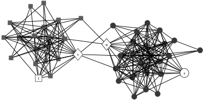
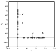
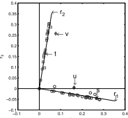
Figure 1: Blue circles are the 25 nodes in one community and red squares are the 20 nodes in the other community. Edges are added across two communities.
2-D case. For a graph with two disconnected communities C1 and C2. All the nodes fromC1 lie on the line that passes through the origin and the point (1, 0) and nodes from C2 lie on the line that passes through the origin and the point (0, 1). We show a synthetic graph with two disconnected communities in Figure 1(a). The solid lines are links within each community. Figure 1(b) shows the spectral coordinates in the 2-D scatter plot when the two communities are disconnected. We can see that all nodes lie along the two axes.
3.2 Spectral Properties of Observed Graphs
Based on Theorem 1, we derive the approximation of the perturbed spectral coordinate αu, which is determined by the original spectral coordinate of itself and that of its neighbors in other communities.
y 2
Theorem2. Denote an observed graph as ˜ A = A+E where A is as shown in (6) and E denotes the edges across communities. For a node u ∈ Ci, let Γju denote its neighbors in Cj for j ̸= i, and Γiu = ∅. The spectral coordinate of u can be approximated as
where scalar xiu is the only non-zero entry in its original spectral coordinate shown in (7), euv is the (u, v) entry of E, and ri is the i-th row of the following matrix
Proof. With Theorem 1, the leading k eigenvectors of ˜ A can be approximated as
Putting the k columns together, we have
Note that when A can be partitioned as in (6), and the original coordinate αu has only one non-zero entry xiu as shown in (7), the u-th row of (˜xi, · · · , ˜xk) in (10) can be simplified as:
Note that euv in the right hand side (RHS) of (8) can be further removed since euv = 1 in our setting. We include euv there for extension to general perturbations. Our next result shows that spectral coordinates also locate along k quasiorthogonal lines ri (the i-th row of R), instead of exactly on the axes ξi when the graph is disconnected.
˜
Proposition 2. For a graph A = A+E, spectral coordinates form k approximately orthogonal lines. Specifically, for any node u ∈ Ci, if it is not directly connected with other communities, αu lies on the line ri; otherwise, αu deviates from lines ri (i = 1, · · · , k), where ri is the i-th row of matrix R shown in Equation (9).
Proof. First we prove that node u ∈ Ci locates on the line ri. When node u has no connections to other communities, the second part of the RHS of (8) is 0. Hence αu ≈ xiuri. When node u has some connections outside Ci, the second part of its spectral coordinate in (8) is not equal to 0, and it thus deviates from line ri.
Next we prove that lines ri are approximate orthogonal. Let W = R - I, then W T + W = 0 since βij = βji. Hence RT R = (I + W T )(I + W) = I - W T W. The (i, j) entry of matrix W T W is ∑t̸ =i,j βit λt-λi βtj λj-λt . Note that the conditions of Theorem 1 imply that βit = xTi Ext is much smaller than |λt - λi|, and hence W T W ≈ 0. Then, RT R ≈ I, and we prove the orthogonality property.
2-D case. Nodes from C1 lie along line r1, while nodes from C2 lie along line r2, where
Note that r1 and r2 are orthogonal since r1rT 2 = 0. For nodes that have connections to the other community, e.g., nodes u and v shown in Figure 1(a), their spectral coordinates scatter between two lines. For node u, its spectral coordinate can be approximated as
Its spectral coordinate jumps away from line r1. The magnitude of jump is determined by spectral coordinates of its connected nodes in the community C2, as shown by the second parts of RHS of (11). Since the jump vector is nonnegative, node u gets closer to line r2. Similarly, we can see for node v jumps towards line r1. In Figure 1(c), we can also see that both r1 and r2 rotate clockwisely from the original axes. This is because β12 = xT1 Ex2 = ∑i,j eijx1ix2j > 0. There is a negative angle θ between line r1 and x-axis since tanθ = β12 λ2-λ1 < 0.
3.3 Laplacian and Normal Eigenspaces
Our perturbation framework based on the adjacency eigenspace utilizes the eigenvectors of the largest k eigenvalues, which are generally stable (due to large eigen-gaps) under perturbation. The line orthogonality property shown in Theorem 2 and Proposition 2 is based on the approximation shown in Theorem 1. Recall that Theorem 1 is derived from Lemma 1 that involves two conditions. These two conditions are naturally satisfied if the eigen-gap of any k leading eigenvalues is greater than 3‖E‖2 (‖E‖2 is the largest eigenvalue of E), which guarantees the relative smaller change and the order of the eigenvectors preserved after perturbation. For condition 1, it is easy to verify that ‖xTi Exi‖2 = 0. Since ‖U T EU‖2 ≤ ‖E‖2 for graph A with k disconnected comparable communities, the condition holds when the eigengap λi - λi+1 is greater than ‖E‖2. For condition 2, we can see ‖U T Exi‖2 is also much smaller than ‖E‖2. Hence, condition 2 is satisfied when the eigengap λi -λi+1 is greater than 3‖E‖2. Note that ‖E‖2 is bounded by the maximum row sum of E and tends to be small when the perturbation edges are randomly added.
Next we examine the spectral spaces of the Laplacian matrix and the normal matrix and explain why the line orthogonality does not hold in their eigenspaces. The Laplacian matrix L is defined as L = D-A, where D = diag{d1, . . . , dn} and di is the degree of node i. The normal matrix N is defined as N = D1 2 AD12 . We can easily derive that, for the blockwise diagonal graph, the spectral coordinate of node u ∈ Ci in the Laplacian eigenspace is (0, . . . , 1, . . . , 0) where the ith entry is 1, indicating the node u's community whereas the coordinate in the normal eigenspace is (0, . . . , √du, . . . , 0). Note that the k eigenvectors corresponding to the smallest eigenvalues of L capture the community structure. However, Lemma 1 is not applicable to ˜ L in general under perturbation, because the gap between the k smallest eigenvalues and the rest ones is too small and the two conditions in Lemma 1 are violated. For the normal matrix, all the eigenvalues of N are between 1 and -1. The conditions in Lemma 1 do not hold either because the eigen-gaps is generally smaller than ‖ΔN‖2. Hence it is impossible to explicitly express the perturbed spectral coordinates using the original ones and the perturbation matrix in the Laplacian or normal eigenspace. As a result, the line orthogonality disappears in the Laplacian or the normal eigenspace.
4 Adjacency Eigenspace based Clustering
In this section, we present a community partition algorithm, AdjCluster, which utilizes the line orthogonality pattern in the spectral space of the adjacency matrix. When a graph contains k clear communities, there exist k quasi-orthogonal lines in the k-dimensional spectral space and each line corresponds to a community in the graph. The spectral coordinate αu should be close to the line corresponding to the community that the node u belongs to. In general, the idea of fitting k orthogonal lines directly in the k-dimensional space is complex. As shown in Algorithm 1, we project each spectral coordinate αu to the unit sphere in the k-dimensional subspace by normalizing αu to its unit length (line 3). We expect to observe that nodes from one community form a cluster on the unit sphere. Hence there will be k well separated clusters on the unit sphere. We apply the clustering k-means algorithm on the unit sphere to produce a partition of the graph (line 4).
Algorithm 1 AdjCluster: Adjacency Eigenspace based Clustering
Input: A,K
Output: Clustering results
- 1: Compute x1,. . . ,xK by the eigen-decomposition of A
- 2: for k = 2,. . . , K do
- 3: αu = (x1u, . . . , xku) and ¯αu = αu ‖αu‖ ;
- 4: Apply k-means algorithmon {¯αu}u=1,...,n;
- 5: Compute fitting statistics from k-means algorithm ;
- 6: end for
- 7: Output partitions under k with the best fitting statistics.
To evaluate the quality of the partition and determine the k, we use the classic Davies-Bouldin Index (DBI ) [Davies and Bouldin, 1979]. The low DBI indicates output clusters with low intra-cluster distances and high inter-cluster distances. When the graph contains k clear communities, we expect to have the minimumDBI after applying k-means in the k-dimensional spectral space. We also expect all the angles between centroids of the output clusters are close to 90◦ since spectral coordinates form quasi-orthogonal lines in the determined k-dimensional spectral space. However, in the subspace spanned by fewer or more eigenvectors, the coordinates scatter in the spaces and do not form clear orthogonal lines, hence we will not obtain a very good fit after applying the k-means on the unit sphere.
Calculation of the eigenvectors of an n×n matrix takes in general a number of operations O(n3 ), which is almost inapplicable for large networks. However, in our framework, we only need to calculate the first K eigen-pairs. We can determine the appropriate K as examining the eigen-gaps [Stewart and Sun, 1990]. Furthermore, adjacency matrices in our context are usually sparse. The Arnoldi/Lanczos algorithm [Golub and Van Loan, 1996] generally needs O(n) rather than O(n2 ) floating point operations at each iteration.
5 Evaluation
We use several real network data sets in our evaluation: Political books and Political blogs 1 , Enron 2 , and Facebook dataset [Viswanath et al., 2009]. We also generate two synthetic graphs: Syn-1 and Syn-2. The Syn-1 has 5 communities with the number of nodes 200, 180, 170, 150, and 140 respectively, and each community is generated separately with a power law degree distribution with the parameter 2.3. We add cross community edges randomly and keep the ratio between inter-community edges and inner-community edges as 20% in Syn-1. Syn-2 is the same as the Syn-1 except that we increase the number of links between community C4 and C5 to 80%. As a result, the Syn-2 has four communities.
5.1 Line Orthogonality Property
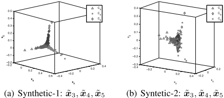
We use spectral scatter plots to check the line orthogonality property in various networks. We learn that for Syn-1 there exist five orthogonal lines in the spectral space. Due to the space limit, we only show the three orthogonal lines (corresponding to communities C3, C4, and C5 denoted by different colors) in the space spanned by ˜x3, ˜x4, ˜x5 in Figure 2(a). For Syn-2, we can observe in Figure 2(b) that there is no clear line orthogonality pattern in the space spanned by ˜x3, ˜x4, ˜x5 since there are actually four communities in Syn-2.
1 http://www-personal.umich.edu/˜mejn/ netdata/
2 http://www.cs.cmu.edu/˜enron/
| Polbooks | Polblogs | Syn-1 | Syn-2 | |
|---|---|---|---|---|
| Adjacency matrix | ||||
| γ | 0.59 | 6.95 | 3.87 | 3.16 |
| δ | 3.08 | 30.8 | 2.44 | 3.23 |
| |λk - λk+1| | 5.82 | 39.6 | 7.65 | 8.26 |
| ‖E‖2 | 2.78 | 13.61 | 6.99 | 6.61 |
| Laplacian matrix | ||||
| γ | 1.54 | 12.1 | 4.10 | 4.11 |
| δ | -11.7 | -73.5 | -23.7 | -25.37 |
| |μk - μk+1| | 0.24 | 0.16 | 0.30 | 0.30 |
| ‖ΔL‖2 | 11.2 | 69.3 | 15.8 | 15.64 |
| Normal matrix | ||||
| γ | 0.144 | 0.15 | 0.24 | 0.27 |
| δ | -0.526 | -0.29 | -1.04 | -1.07 |
| |νk - νk+1| | 0.139 | 0.07 | 0.20 | 0.20 |
| ‖ΔN ‖2 | 0.650 | 0.35 | 0.76 | 0.78 |
Our theoretical analysis in Section 3.3 showed that the orthogonality pattern does not held in either Laplacian or normal eigenspace because their small eigen-gap values affect the stability of the spectral space (Recall the conditions in Lemma 1 and Theorem 1). Table 1 shows the calculated values of γ, δ, eigen-gap, and the magnitude of perturbations in adjacency, Laplacian, and normal eigenspaces for various networks. We can see that for adjacency matrices, all the networks generally satisfy conditions, which explains line orthogonality patterns in their adjacency eigenspaces. However, for Laplacian or normal matrices, none of networks satisfies the conditions. For example, all δ values for Laplacian or normal matrix (shown in bold) are less than zero, violating Condition 1 in Lemma 1; all values of ‖ΔL‖2 or ‖ΔN‖2 (shown in italic) are less than their corresponding eigengaps, incurring the violation of Condition 2 in Lemma 1; and the eigengaps (|μk -μk+1|, |νk -νk+1|) are relatively small, violating the condition in Theorem 1. Hence, the orthogonality pattern does not held in Laplacian or normal eigenspaces (we skip their scatter plots due to space limitations).
5.2 Quality of Community Partition
Table 2 shows the quality of our graph partition algorithm AdjCluster. The algorithm chooses the value of k that incurs the minimumDBI for each network data set. For a network with a clear community structure, we expect that the DBI is small, the modularity is away from zero, and the average angle is close to 90◦ since there exist k quasi-orthogonal lines in the spectral space. We can see from Table 2 that all networks show relatively clear community structures.
The original data descriptions of Polbooks and Polblogs (and Syn-1/Syn-2) provide node-community relations. So we are able to compare different algorithms in terms of accuracy. The accuracy is defined as ∑ki=1 |Ci∩ ˆCi | n where ˆ Ci denotes the i-th community produced by different algorithms. In our experiment, we compare our AdjCluster with four graph partition algorithms: one Laplacian based algorithm (the geometric spectral clustering) [Miller and Teng, 1998], one normal based algorithm (the normalized cut [Shi and Malik, 2000]), one modularity based agglomerative clustering algorithm (HE′ [Wakita and Tsurumi, 2007]), and the EigenSpoke algorithm (SpokEn [Prakash et al., 2010]). Table 3 shows the accuracy values on the above four networks. Note that we cannot report accuracy values for Enron or Facebook since we do not know about their exact true community partitions. We can see that the quality of the partitioning produced by our algorithm AdjCluster is better than (or comparable with) that produced by the normalized cut in terms of accuracy. On the contrary, the Laplacian spectrum based algorithm, the modularity based agglomerative clustering algorithm, and the EigenSpoke algorithm produce significant low accuracy values, which matches our theoretical analysis.
| Dataset | n | m | k | DBI | Angle | Q |
|---|---|---|---|---|---|---|
| Syn-1 | 840 | 4917 | 5 | 0.45 | 80.7◦ | 0.37 |
| Syn-2 | 840 | 5389 | 4 | 0.49 | 76.5◦ | 0.34 |
| Polbooks | 105 | 441 | 2 | 0.15 | 83.8◦ | 0.45 |
| Polblogs | 1222 | 16714 | 2 | 0.17 | 90.4◦ | 0.42 |
| Enron | 148 | 869 | 6 | 0.59 | 88.9◦ | 0.48 |
| 63392 | 816886 | 9 | 0.83 | 83.6◦ | 0.51 |
| Dataset | AdjCluster | Lap | NCut | HE′ | SpokEn |
|---|---|---|---|---|---|
| Syn-1 | 90.8 | 57.5 | 84.4 | 49.1 | 40.2 |
| Syn-2 | 85.1 | 62.8 | 80.1 | 45.9 | 44.7 |
| Polbooks | 96.7 | 93.5 | 96.7 | 88.0 | 93.5 |
| Polblogs | 94.7 | 58.8 | 95.3 | 92.4 | 91.9 |
6 Conclusion and Future Work
In this paper we have demonstrated the line orthogonality in the adjacency eigenspace. Using this orthogonality property, we presented our graph partition algorithm AdjCluster and showed its effectiveness for community partition. Although we mainly focused on theoretical studies of the line orthogonality property in this paper, we believe many applications based on the line orthogonality property could be developed. For example, we could develop adaptive clustering methods using adjacency matrix perturbation for tracking changes in clusters over time. We could also identify bridging nodes by examining outliers from k-means output. Bridging nodes are the nodes connecting to multiple communities. In the spectral space, they are neither close to the origin, nor close to any fitted orthogonal line corresponding to a certain community. Therefore, we could mark a node as a bridging one if its projection in the unit sphere is not close to any centriod. In our future work, we will explore the line orthogonality property in more (and larger) social networks and conduct complete comparisons with other recently developed spectral clustering algorithms (e.g., [Huang et al., 2008]). We also plan to extend our studies to signed graphs which contain both positive and negative edges.
Acknowledgment
This work was supported in part by U.S. National Science Foundation (CCF-1047621, CNS-0831204) for X. Ying, L. Wu, and X. Wu and by NSFC (61073097, 61021062) and JiangsuSF (BK2008018) for Z.-H. Zhou.
@inproceedings{ijcai2011p391,
  title     = {Line Orthogonality in Adjacency Eigenspace with Application to Community Partition},
  author    = {Wu, Leting and Ying, Xiaowei and Wu, Xintao and Zhou, Zhi-Hua},
  booktitle = {Proceedings of the Twenty-Second International Joint Conference on
               Artificial Intelligence, {IJCAI-11}},
  publisher = {AAAI Press/International Joint Conferences on Artificial Intelligence},
  editor    = {Toby Walsh},
  pages     = {2349--2353},
  year      = {2011},
  month     = {7},
  doi       = {10.5591/978-1-57735-516-8/IJCAI11-391},
  url       = {https://doi.org/10.5591/978-1-57735-516-8/IJCAI11-391},
}
TY - CPAPER TI - Line Orthogonality in Adjacency Eigenspace with Application to Community Partition AU - Wu, Leting AU - Ying, Xiaowei AU - Wu, Xintao AU - Zhou, Zhi-Hua T2 - Proceedings of the Twenty-Second International Joint Conference on Artificial Intelligence, IJCAI-11 PB - AAAI Press/International Joint Conferences on Artificial Intelligence PY - 2011 SP - 2349 EP - 2353 DO - 10.5591/978-1-57735-516-8/IJCAI11-391 UR - https://doi.org/10.5591/978-1-57735-516-8/IJCAI11-391 ER -Copied
Machine-readable versions of this paper, for tools and AI agents:





