
New Complexity Results for MAP in Bayesian Networks
Proceedings of the Twenty-Second International Joint Conference on Artificial Intelligence. Pages 2100-2105.
https://doi.org/10.5591/978-1-57735-516-8/IJCAI11-351
© 2011 International Joint Conferences on Artificial Intelligence
Abstract
This paper presents new results for the (partial) maximum a posteriori (MAP) problem in Bayesian networks, which is the problem of querying the most probable state configuration of some of the network variables given evidence. It is demonstrated that the problem remains hard even in networks with very simple topology, such as binary polytrees and simple trees (including the Naive Bayes structure), which extends previous complexity results. Furthermore, a Fully Polynomial Time Approximation Scheme for MAP in networks with bounded treewidth and bounded number of states per variable is developed. Approximation schemes were thought to be impossible, but here it is shown otherwise under the assumptions just mentioned, which are adopted in most applications.
- [Bodlaender, 1993] H. L. Bodlaender. A linear time algo- rithm for finding tree-decompositions of small treewidth. In Proc. of STOC, pages 226-234, 1993. ACM.
- [Darwiche, 2009] A. Darwiche. Modeling and Reasoning with Bayesian Networks. Cambridge Univ. Press, 2009.
- [Garey and Johnson, 1979] M. R. Garey and D. S. Johnson. Computers and Intractability: A Guide to the Theory of NP-Completeness. W. H. Freeman, 1979.
- [Papadimitriou and Yannakakis, 2000] C. H. Papadimitriou and M. Yannakakis. On the approximability of trade-offs and optimal access of web sources. In Proc. of FOCS, page 86-92, 2000. IEEE Computer Society.
- [Park and Darwiche, 2004] J. D. Park and A. Darwiche. Complexity results and approximation strategies for MAP explanations. J. Artif. Intell. Res., 21:101-133, 2004.
- [Pearl, 1988] J. Pearl. Probabilistic Reasoning in Intelligent Systems: Networks of Plausible Inference. Morgan Kauf- mann, 1988.
- [Shenoy, 1996] Prakash P. Shenoy. Binary join trees. In Proc. of UAI, pages 492-499, 1996.
- [Vazirani, 2001] V. V. Vazirani. Approximation Algorithms. Springer, 2001.
References were extracted automatically from the PDF and may contain errors.
Full text extracted automatically from the PDF; figures, tables and equations may differ. The PDF is the version of record.
1 Introduction
A Bayesian network (BN) is a probabilistic graphical model that relies on a structured dependency among random variables to represent a joint probability distribution in a compact and efficient manner. One of the hardest inference problems in BNs is the maximum a posteriori (or MAP) problem, where one looks for states of some variables that maximize their joint probability, given some other variables as evidence (there may exist variables that are neither queried nor part of the evidence). This problem is known to be NP PP - complete in the general case and NP-complete for polytrees [Park and Darwiche, 2004]. Thus, algorithms usually take large amount of time to solve MAP even in small networks. Approximating MAP in polytrees is also NP-hard. However, such hardness results are derived for networks with a large number of states per variable, which is not the most common situation in many practical problems. In this paper, a bounded number of states per variable is considered. It is proven that the problem remains hard even in binary polytrees and simple trees, using reductions from both the satisfiability and the partition problems, but it is also shown that there is a Fully Polynomial Time Approximation Scheme (FPTAS) whenever treewidth and number of states are bounded, so one may expect fast algorithms for MAP with a small approximation error under such assumptions. Fast algorithms for MAP may imply in fast algorithms for other related problems, for example inferences in decision networks and influence diagrams, besides the great interest in the MAP problem itself. Hence, this paper makes important steps in these directions.
2 Background
The reader is assumed to be familiar with basic notions of complexity theory and approximation algorithms (for example, see [Garey and Johnson, 1979; Vazirani, 2001]) and basic concepts of Bayesian networks [Pearl, 1988].
Definition 1 A Bayesian network (BN) N is a triple (G, X, P), where G = (VG, EG) is a directed acyclic graph with nodes VG associated (in a one-to-one mapping) to random variables X = {X1, . . . ,Xn} over discrete domains {ΩX1 , . . . , ΩXn } and P is a collection of probability values p(xi|πXi ) ∈ Q, 1 with ∑xi∈ΩXi p(xi|πXi ) = 1, where xi ∈ ΩXi is a category or state of Xi and πXi ∈ ×X∈PAXi ΩX a complete instantiation for the parents PAXi of Xi in G. Furthermore, every variable is conditionally independent of its non-descendant non-parents given its parents.
The joint probability distribution represented by a BN (G,X,P) is obtained by p(x) = ∏i p(xi|πXi ), where x ∈ ΩX and all states xi, πXi (for every i) agree with x. Now we introduce some notation. Singletons {Xi} and {xi} are respectively denoted as Xi and xi. Nodes of the graph and their associated random variables are used interchangeably. Uppercase letters are used for random variables and lowercase letters for their corresponding states. Bold letters are employed for vectors/sets. z(X) denotes the product of the cardinality of the variables X ⊆ X, that is, z(X) = ∏Xi∈X |ΩXi | (with z(∅) = 1). The input size S(N) of a BN is given by the length of the bit string to specify all the local conditional probability distributions and the structure to describe the graph. Note that S(N) ≥ n and S(N) ≥ zmax = maxXi∈X z(Xi).
The belief updating (BU) problem concerns the computation of p(x|e), for x ∈ ΩX and e ∈ ΩE, with X∪E ⊆ X and X∩E = ∅. The complexity of solving BU is tightly related to the minimum treewidth of the network, or maximum number of variables in a single node of the most compact tree decomposition (for example, see [Darwiche, 2009]). In spite of that, some particular BNs deserve attention: N = (G,X,P) is called a polytree if the subjacent graph (dropping the direction of the arcs) of G has no cycles. A polytree N is further called a tree if each node of G has at most one parent. The treewidth of a tree is one. For trees and polytrees, BU is solvable in polynomial time [Pearl, 1988]. This is also true for any network of bounded treewidth. Finding a tree decomposition of minimum treewidth is hard, but it is enough to know a bound for the treewidth (which is not part of the input) to obtain it in polynomial time [Bodlaender, 1993].
1Q denotes the non-negative rational numbers defined by fractions of integers.
The MAP problem is to find an instantiation xopt ∈ ΩX map , with X map ⊆ X \ E, such that its probability is maximized:
because p(e) (assumed to be non-zero 2 ) is a constant with respect to the maximization. It is known that MAP queries are harder than BU queries (under the assumptions that P̸=NP and PP̸=NP PP ). It is proven that the general MAP problem is NP PP -complete [Park and Darwiche, 2004]. However, such proof assumes a general case of the problem, while many practical BNs have some structural properties that might alleviate the complexity. Two of them are very important with respect to the complexity of the problem: the cardinality of the variables involved in the network and the minimum treewidth. The latter is considered in [Park and Darwiche, 2004], and the problem is shown to be NP-complete and not approximable by a polynomial approximation scheme even if the treewidth is bounded. In this paper both treewidth and cardinality of the network are exploited, which allows us to go further in the analysis.
Definition 2 Given a BN N = (G, X , P) such that the maximum cardinality of any variable is at most z and the minimum treewidth is at most w, X ⊆ X \ E, a rational r and an instantiation e ∈ ΩE, Decision-MAP-z-w is the problem of deciding if there is x ∈ ΩX such that p(x, e) > r. MAP-z-w is the respective optimization version.
3 Complexity results
Hardness of MAP is known for polytrees where the maximum cardinality of a variable is Θ(S(N)) [Park and Darwiche, 2004]. More specifically, Decision-MAP-∞-w, where ∞ is used to indicate that there is no bound for z, is known to be NP-hard for w = 2, because the cardinality of the network used in the proof could be as large as the number of clauses in the SAT problem used in the reduction, and this number can be asymptotically as large as the SAT input size. It was also shown that Decision-MAP-z-∞ is NP-hard for z = 2. The next theorem strengthen those two results.
Theorem 3 Decision-MAP-z-w is NP-hard even if z = w = 2.
2 If p(e) is zero, then so is p(x, e), and the problem vanishes, as any x will be a maximizer for the problem.
Proof Hardness is shown using a reduction from partition problem, which is NP-hard [Garey and Johnson, 1979] and can be stated as follows: given a set of m positive integers s1, . . . , sm, is there a set I ⊂ A = {1, . . . ,m} such that ∑i∈I si = ∑i∈A\I si? All the input is encoded using b > 0 bits. Denote S = 12 ∑i∈A si and call even partition a subset I ⊂ A that achieves ∑i∈I si = S. To solve partition, one may consider the rescaled problem (dividing every element by S), so as vi = si S ≤ 2 are the elements and the goal is a partition I with sum equals to 1.
A binary polytree (so zmax = 2) with 3m+ 1 nodes, maximum number of parents per node equals to 2, and treewidth w = 2 is built in polynomial time. The binary nodes are X = {X1, . . . ,Xm}, Y = {Y0, Y1, . . . , Ym} and E = {E1, . . . ,Em}. We denote by {xTi , xFi } the states of Xi (similarly for Yi and Ei). The structure of the network is presented in Figure 1. Each Xi ∈ X has no parents and uniform distribution, each Ei has Xi as sole parent, with probability values defined as p(eTi |xFi ) = 1 and p(eTi |xTi ) = ti (the values for eFi complement those of eTi ), where ti is obtained by evaluating 2-vi up to 4b + 3 bits of precision and by rounding it up (if necessary), that is, ti = 2-vi + errori, where 0 ≤ errori < 2-(4b+3) . Clearly ti can be computed in polynomial time and space in b (this ensures that the specification of the Bayesian network, which requires rational numbers, is polynomial in b). Furthermore, note that 2-vi ≤ ti ≤ 2-vi + errori < 2-vi + 2-(4b+3) ≤ 2-vi+2-4b (in short, this holds because 2-4b in the exponent makes the value grow faster than the linear addition of 2-(4b+3) . Further details are omitted for simplicity).
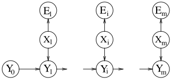
Y0 has no parents and p(yT 0 ) = 1. For the nodes Yi ∈ Y, 1 ≤ i ≤ m, the parents are Xi and Yi-1, and the probability values are p(yT i |yT i-1 , xTi ) = ti, p(yT i |yT i-1 , xFi ) = 1, and p(yT i |yF i-1 , xi) = 0 for both states xi ∈ ΩXi .
Note that with this specification and given the Markov condition of the network, we have (for any given x ∈ ΩX) p(yTm|x) = p(eT|x) = ∏i∈I ti, where I ⊆ A is the set of indices of the elements such that Xi is at the state xTi . Denote t = ∏i∈I ti. Then p(x, eT, yFm) = p(yFm|x)p(x, eT) = p(x)p(eT|x) (1 -p(yTm|x)) = 1 2m t(1 - t). This is a concave quadratic function on 0 ≤ t ≤ 1 with maximum at 2-1 such that t(1-t) monotonically increases when t approaches one half (from both sides). If ti was exactly 2-vi , then 1 2m t(1 -t) = 1 2m 2- ∑i∈I vi (1 - 2- ∑i∈I vi ), which achieves themaximumof 1 2m 2-1 (1 - 2-1) if and only if ∑i∈I vi = 1, that is, if there is an even partition. However 2-vi is used with
4b + 3 bits of precision to ensure the computation is done in polynomial time, so the remainder of this proof addresses the question of how the numerical errors introduced in the definition of values ti interfere in the main result. Hence, note that if I is not an even partition, then we know that one of the two conditions hold: (i) ∑i∈I si ≤ S - 1 ⇒ ∑i∈I vi ≤ 1 - 1S , or (ii) ∑i∈I si ≥ S + 1 ⇒ ∑i∈I vi ≥ 1 + 1S , because the original numbers si are integers. Consider these two cases.
by using S ≤ 2b and m ≤ b < 2b . On the other hand, if ∑i∈I si ≤ S - 1, then t ≥ ∏i∈I 2-vi equals to
Now suppose I ′ is an even partition. Then we know that the corresponding t′ satisfies 2-1 ≤ t′ and
To complete the proof, we show that the distance between t′ and 2-1 is always less than the distance between t and 2-1 of a non-even partition plus a gap, that is,
which can be proved by analyzing the two elements of the min. The first term holds because
The second comes from the fact that the function h(b) = a + l + 2-(3b+2) = 2-1+ 1 23b + 2-1-( 1 2b - 1 23b ) + 2-(3b+2) is less than 1 for b = 1, 2 (by inspection), it is a monotonic increasing function for b ≥ 2 (the derivative is always positive), and it has limb→∞h(b) = 1. Hence, we conclude that h(b) < 1, which implies
This concludes that there is a gap of at least 2-(3b+2) between the worst value of t′ (relative to an even partition) and the best value of t (relative to a non-even partition), which will be used next to specify the threshold of the MAP problem. Now, set up X to be the MAP variables and E = e, Ym = yFm to be the evidence, so as the MAP decision becomes
where c is defined as a′ · (1-a′), with a′ equals a evaluated up to 3b + 2 bits and rounded up, which implies that 2-1 < a ≤ a′ < a+2-(3b+2). By Eq. (2), a′ is closer to one half than any t of a non-even partition, so the value c is certainly greater than any value that would be obtained by a non-even partition. On the other hand, a′ is farther from 2-1 than a, so we can conclude that c separates even and non-even partitions, that is, t·(1-t) < c ≤ a·(1-a) < t′ ·(1-t′ ) for any t corresponding to a non-even partition and any t′ of an even partition. Thus, a solution of the MAP problem obtains p(x, eT, yFm) > r if and only there is an even partition. 3 □
Corollary 4 Decision-MAP is NP-complete when restricted to binary polytrees.
Proof It follows directly from Theorem 3 and the wellknown fact that Decision-MAP is in NP when w is fixed. □
The next theorem shows that the problem remains hard even in trees. The tree used for the proof is probably the simplest practical tree: a Naive Bayes structure, where there is a node called class with direct children called features. These features are independent of each other given the class. The simplicity of this tree makes the result stronger. Moreover, by reducing from the maximum-satisfiability problem, we show later that the inapproximability results before known for polytrees [Park and Darwiche, 2004] (when the maximum cardinality is not bounded) extend to the case of trees.
Theorem 5 Decision-MAP-∞-w is NP-hard if w = 1 and the network topology follows the Naive Bayes structure.
Proof We use a reduction from MAX-2-SAT. Let X1 . . . ,Xm be variables of a SAT problem with clauses C1, . . . ,Cm′ written in 2CNF, that is, each clause is composed of a disjunction of two literals. Each literal belongs to ΩXj = {xj, ¬xj} for a given j. Without loss of generality, we assume that each clause involves exactly two distinct variables of X1 . . . ,Xm. Let b > 0 be the number of bits to specify the MAX-2-SAT problem.
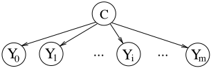
Take a Naive Bayes shaped network. The idea is to build a network where the features represent the SAT variables and the class represents ways to satisfy the clauses, such that summing over the class states will produce the number of satisfying clauses. This is performed by considering the left and right literals of each clause in three conditions: (i) the clause is satisfied by its left literal (in this case, the value of the right literal is ignored), (ii) the clause is not satisfied by its left literal, but it is by its right literal, (iii) the clause is not satisfied by either of them. Therefore, Let C be the root of the Naive Bayes structure and Y1, . . . , Ym the binary features (as shown in Figure 2) such that ΩYj = {yT j , yF j } for every j. Define the variable C to have 2m′ states and uniform prior, that is, p(c) = 1 2m′ for every c ∈ ΩC, where
3 The conditional version of Decision-MAP could be used in the reduction too by including the term 1 p(eT,yFm) in r, which can be computed in polynomial time by a BN propagation in polytrees [Pearl, 1988], and it does not depend on the choice x.
ΩC equals to {c1L, c1R, c2L, c2R, . . . , cm′L, cm′R}. Denote by Li the literal of clause Ci with the smallest index, and by Ri the literal with the greatest index. Define the conditional probability functions of each Yj given C as follows: p(yT j |ciL) = p(yT j |ciR) = 12 if Li,Ri /∈ ΩXj , that is, Xj does not appear in clause Ci, p(yT j |ciR) = 1 if (xj = Ri) ∨ (¬xj = Li), p(yT j |ciR) = 0 if (xj = Li) ∨ (¬xj = Ri), p(yT j |ciL) = 1 if (xj = Li), p(yT j |ciL) = 0 if (¬xj = Li), p(yT j |ciL) = 1 2 if Ri ∈ ΩXj . Define Y0 as an extra feature such that p(yT 0 |ciL) = 1 and p(yT 0 |ciR) = 1/2 for every i. The probability values for yF j complement these numbers, that is, p(yF j |c) = 1 - p(yT j |c) for every c ∈ ΩC. Hence, maxy0...ym p(y0, y1, . . . , ym) = maxy1,...ym p(yT 0 , y1, . . . ym), because the vector p(yT 0 |C) has p(yT 0 |c) ≥ p(yF 0 |c) for every c ∈ ΩC (there is no reason to choose yF 0 in place of yT 0 as the probability value of the latter is always greater than that of the former for every given c). It is clear that the transformation is polynomial in b, as the network has m+1 nodes, with at most 2m′ states (both m and m′ are O(b)), and the probability values are always 0, 1/2 or 1. By simple manipulations, we have
where jiL and jiR, with jiL < jiR, are the indices of the two variables that happen in clause Ci (the probability of all other variables Yj that appeared in the product have led to the fraction 12 because they do not happen in Ci and hence disappeared to form the constant 1 2m-2 that has been put outside the summation). Yet by construction, p(yT , y1, . . . ym) =
0
Note that p(yjiL |ciL) = 1 if and only if p(yjiL |ciR) = 0 (and p(yjiL |ciL) = 0 if and only if p(yjiL |ciR) = 1), and p(yjiL |ciL) = 1 if and only if the instantiation of the Boolean variable in Li satisfies clause Ci. In this case, p(yjiL |ciR) = 0, and the sum p(yjiL |ciL) + p(yjiL |ciR)p(yjiR |ciR) equals to 1. On the other hand, if the Boolean variable in Li does not make clause Ci satisfiable, then p(yjiL |ciL) + p(yjiL |ciR)p(yjiR |ciR) = p(yjiR |ciR), that is, it is one if and only if the Boolean in Ri satisfies Ci. Because we sum over all clauses, p(yT 0 , y1, . . . ym) = k 2mm′ ⇐⇒ k clauses are satisfiable. Hence, solving maxy0...ym p(y0, y1, . . . , ym) is the same as solving MAX-2-SAT, and the reduction of the decision version easily follows. □
We show next a stronger inapproximability result than previously stated in the literature, because we make use of trees instead of polytrees. Recall that an approximation algorithm for a maximization problem where the exact maximum value is M > 0 is said to achieve a ratio α > 1 from the optimal if the resulting value is guaranteed to be greater than or equal to Mα . We demonstrate that approximating MAP is NP-hard even if the network topology is as simple as a tree. This leaves no hope of approximating MAP in polynomial time when the number of states per variable is not bounded.
Theorem 6 It is NP-hard to approximate MAP-∞-w, with w = 1, to any ratio α = 2S(N)ε , for fixed 0 ≤ ε < 1.
Proof We show that it is possible to reduce MAX-2-SAT to the approximate version of MAP-∞-1 in polynomial time and space in the size of input. The idea is similar to the repeated construction used in [Park and Darwiche, 2004]. We build q copies of the network of Theorem 5 (superscripts are added to the variables to distinguish the copies as follows: the nodes of the t-th copy are named Ct , Y t 0 , . . . , Y tm) and link them by a common binary parent D of all the Ct nodes (as shown in Fig.3), with states {dT , dF }. We define p(dT ) = 1 and p(ct |dT ) remains uniform as before, for every node Ct .
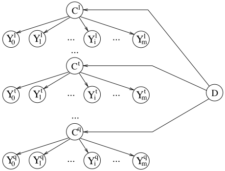
By construction, we have p(y1 0 , . . . y1m, . . . , yq 0 , . . . yqm) =
and hence each copy has independent computations given dT . By the argument in the proof of Theorem 5 for each copy, we obtain p(y1 0 , . . . y1m, . . . , yq 0 , . . . yqm) = ∏qt=1 p(yt0 , . . . ytm) = ∏qt=1 k 2mm′ = ( k 2mm′ )q if and only if k clauses are satisfiable in the MAX-2-SAT problem. Suppose we want to decide if at least 1 < k′ ≤ m′ clauses are satisfiable (the restriction of k′ > 1 does not lose generality). Using the approximation over this new network with ratio α, if at least k′ clauses are satisfiable, then we must have p(y1 0 , . . . y1m, . . . , yq 0 , . . . yqm) ≥ 1α ( k′ 2mm′ )q . On the other hand, if it is not possible to satisfy k′ clauses, then we know that p(y1 0 , . . . y1m, . . . , yq 0 , . . . yqm) ≤ ( k′-1 2mm′ )q . Now we need to show that it is possible to pick q such that ( k′-1 2mm′ )q < 1α ( k′ 2mm′ )q and such that q is polynomially bounded. The proof concludes by choosing a q such that q > (log(2)k′f ′ (b)ε ) 1 1-ε , which is polynomial in the input size (b is the input size of MAX-2-SAT and f ′ is the size of one of the Naive Bayes structures) and implies q > log(2)k′ qε · f ′ (b)ε =⇒ q > k′ log(2(q·f ′ (b))ε ) =⇒ q > k′ log(2S(N )ε ) =⇒ q > k′ log(α). By Taylor expansion we have log ( k′ k′-1 ) ≥ 1 k′ (for any k′ > 1) and thus q > k′ log(α) =⇒ q > log(α) log( k′ k′ -1 ) =⇒ (k′ - 1)q < 1α (k′ )q =⇒ ( k′ -1 2mm′ )q < 1α ( k′ 2mm′ )q . □
Theorem 7 shows that, even with bounded cardinality and very simple trees, it is hard to solve MAP. The construction that is used in the proof is trick, aiming at Eq. (4), which has the product of values ti from the partition problem (as in Theorem 3) appearing in a competing way in the equation.
Theorem 7 Decision-MAP-z-w is NP-hard even if z = 5 and w = 1 and the network topology follows a Hidden Markov Model (HMM) structure.
Proof This proof uses the exact same rescaled partition problem of the proof of Theorem 3, as well as the idea of approximating exponentials to guarantee that the reduction is polynomial (refer there for the definition of the problem).
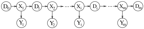
We construct (in polynomial time) a tree with 3m + 1 nodes: X = {X1, . . . ,Xm}, Y = {Y1, . . . , Ym} and D = {D0, D1, . . . , Dm}, such that ΩXi = {xi1, xi2, xi3, xi4, xi5} has 5 states, ΩYi = {yT i , yF i } is binary, and ΩDi = {dTi , dFi , d∗i } is ternary. The structure of the network is presented in Figure 4. The probability functions are defined by Table 1 (except for D0, which has uniform distribution).
First, we show that p(y) = p(y1, . . . , ym) = 1 2m for any configuration y ∈ ΩY. By construction, we have p(yi|di-1) = ∑xi p(yi|xi)p(xi|di-1) = 1 2 for any value of yi, di-1. Now,
Applying the same idea successively, we obtain p(y1, . . . , ym) = 1 2m . Using a similar procedure, we can obtain the values for p(dTm, y) and p(dFm, y) as follows:
and applying successively, we get p(dTm, y) = 2-m 3 ∏i∈I ti, where I ⊂ A is the set of indices of elements such that Yi is at the state yT i (the ratio 13 comes from the uniform p(D0)). Likewise,
| p(Yi|Xi) | xi1 | xi2 | xi3 | xi4 | xi5 |
|---|---|---|---|---|---|
| yi | 1 | 1 | 0 | 0 | 1/2 |
| ¬yi | 0 | 0 | 1 | 1 | 1/2 |
| p(Xi|Di-1) | dTi-1 | dFi-1 | d∗i-1 | ||
| xi1 | 1/2 | 0 | 0 | ||
| xi2 | 0 | 1/2 | 0 | ||
| xi3 | 0 | 1/2 | 0 | ||
| xi4 | 1/2 | 0 | 0 | ||
| xi5 | 0 | 0 | 1 | ||
| p(Di|Xi) | xi1 | xi2 | xi3 | xi4 | xi5 |
| dTi | ti | 0 | 0 | 1 | 0 |
| dFi | 0 | 1 | ti | 0 | 0 |
| d∗i | 1 - ti | 0 | 1 - ti | 0 | 1 |
and again p(dFm, y) = 2-m 3 ∏i∈A\I ti. Therefore,
Consider that ti = 2-vi . The function ∏i∈I ti+∏i∈A\I ti = 2- ∑i∈I vi + 2- ∑i∈A\I vi is convex and achieves its minimum when 2- ∑i∈I vi = 2- ∑i∈A\I vi ⇐⇒ ∑i∈I vi = ∑i∈A\I vi = 1. Thus, using Y as the MAP variables and d∗m as the evidence, we obtain maxy p(d∗m, y) = 23 1 2m if and only if there is an even partition. This is still flaw in one respect: the specification of the network depends on computing ti, for each i ∈ A, which can be done only to a certain precision (we can only use a number of places that is polynomial in b). The derivation follows in a similar way as done in Theorem 3, but using 6b + 3 bits of precision. □
Corollary 8 Decision-MAP is NP-complete when the graph is restricted to a tree and variables have bounded cardinality.
Proof It follows directly from Theorem 7 and the fact that Decision-MAP is in NP when w is fixed. □
Despite the hardness results, we obtain a fully polynomialtime approximation scheme when cardinality and treewidth are bounded. For this purpose, algorithms for BU can be seen as a way to represent and compute a polynomial function on the probability values that define the network. The idea to approximate MAP is that we can iteratively use an inference algorithm for BU, but computing the polynomial for every possible configuration of the query variables X map . As there are too many instantiation of X map , we check at every intermediate step of the algorithm for options xmap that are close to each other, so that the error of using one or another is below some threshold. In this case, we discard options as soon as possible and keep only a polynomial number of them, that are enough to approximate well the result.
Theorem 9 MAP-z-w has a FPTAS for any fixed z and w.
Proof We construct an approximation algorithm A that, for a given ε > 0, is polynomial in S(N) and in 1ε such that the value pA(xmap , e) obtained by A is at least p(xmap opt ,e) 1+ε , where p(xmap opt , e) stands for the optimal solution value of MAP-zw, that is, xmap opt = argmaxxmap p(xmap , e). We know that p(xmap opt , e) > 0 because ∑xmap p(xmap , e) = p(e) > 0 and thus the value achieving the maximum cannot be zero (p(e) > 0 does not lose generality, as discussed before).
Take a binary tree decomposition ({C1, . . . , Cn′ }, T ) with treewidth (at most) w, such that n′ ≤ 2n and Cj indicates both a node of the tree T and the set of network variables associated to that node, which can be obtained in polynomial time [Bodlaender, 1993; Shenoy, 1996]. Let w′ = w + 1 be a bound for the maximum number of variables in a single node of the decomposition. Elect a node and assume all edges of T point towards the opposite direction of it. Without loss of generality, let C1 be this node and C1, . . . , Cn′ be a topological order with respect to this tree. Let Cjp = PACj be the only parent of Cj in the tree and ΛCj be the children of Cj .
Let Xlast j = Cj \ Cjp be the set of nodes of G in Cj that do not appear in the parent Cjp (they also do not appear in any other node towards C1 because of the properties of a tree decomposition). To solve BU, we can use the following recursion, which is processed from j = n′ to 1: p(uCj |vCj ) =
and Xproc j = {Xi ∈ (Cj \ ⋃Cj′∈ΛCj UCj′ ) : (Xi ∪PAXi )∩ Xlast j ̸= ∅} is the set of variables whose local probability functions were not processed yet (but need to be) in order to sum out over Xlast j \X′ (X′ are the variables whose states are fixed). Furthermore, UCj is composed of elements of Cj and descendants that are also present in the parent Cjp and whose local probability distributions were already taken into account (they do appear in the left side of the conditioning bar in a potential in Cj or in its descendants), and finally VCj are the variables that already appeared in the right side of the conditioning bar (but not in the left side nor they were summed out). Note that Eq. (5) is computed for every uCj and every vCj . Each step j can be seen as one bucket in the bucket elimination algorithm (apart from the fact that we might sum out more than one variable at once - this can also be implemented in the bucket elimination), or the processing of a node in a join tree algorithm. In fact, the values p(uCj′ |vCj′ ) that come from previous computations represent the information from the children of Cj, with domains ΩUCj′ ∪VCj′ that come from independent subtrees, and are used to construct p(uCj |vCj ) over ΩUCj ∪VCj . The recursion is evaluated for each j, and finally p(uC1 ) = p(x′ ), where x′ are the fixed states of X′ . The running time, in number of additions and multiplications, is at most ∑j (1 + |ΛCj |) · z(Cj) ∈ O(n · zwmax) ∈ O(n), as both zmax and w = maxj |Cj | are bounded.
To solve the MAP problem, the evidence e is considered part of x′ , and Eq. (5) is computed for every distinct instantiation of the MAP variables that have already appeared in a given subtree. The tree is iteratively processed until the root is reached. We use the notation pxmap C (u|v) = p(u|v) such that u and v agree with xmap C , where xmap C ∈ ΩXmap C (and Xmap C ⊆ X map ), to indicate that the MAP variables that appear in a subtree rooted at C are fixed to the value xmap C and hence this can be interpreted as having distinct potentials pxmap C for distinct instantiations xmap C . Note that pxmap C has d = z((U∪V) \ (E ∪ Xmap C )) elements as arguments (the part of u, v corresponding to e and xmap C are fixed). With this approach, we can rewrite Eq. (5) to introduce the MAP variables just by replacing p with pxmap Cj , where xmap Cj is restricted to the variables that already appeared in the computation (and further supposing that Xmap Cj is never summed out). This algorithm is correct, but it eventually has to process an exponential number of potentials pxmap Cj (one for each xmap Cj ), because as the algorithm goes on, as the set of already processed MAP variables increases, until the MAP variables are again altogether in the root.
To overcome this situation, we devise a criterion to keep only potentials that are reasonably apart. Notice now that 1 ≥ p(e) ≥ p(xmap opt , e) > 2-g(S(N)) , where g is a polynomial function, because p(xmap opt , e) is obtained from a sequence of additions and multiplications through Eq. (5) over numbers of the input. The same argument holds for every intermediate probability value that is computed through Eq. (5): we have that pxmap Cj (uCj |vCj ) > 0 ⇒ pxmap Cj (uCj |vCj ) > 2-g(S(N)) , for a given polynomial function g. Hence, let g be a polynomial function that satisfies such condition for every number involved in the calculations. Because each pxmap Cj (UCj |VCj ) can be represented by a vector in the dimension d = z((UCj ∪ VCj ) \ (E ∪ Xmap Cj )), the idea is to show that we can fix an upper bound to the number of candidates pxmap Cj (UCj |VCj ) that are propagated from one step to the next. Following the ideas of [Papadimitriou and Yannakakis, 2000], we divide the hypercube [2-g(S(N)) , 1]d into a lattice of hypercubes such that, in each coordinate, the ratio of the largest to the smallest value is 1 + ε 2w′n′ , which produces a number of hypercubes bounded by
where the log appears because the lattice is created from 1 to
2-g(S(N)) , successively dividing the coordinate by 1 + ε 2w′ n′ (a bin for the exact zero probability is also allocated). In each of these smaller hypercubes, we keep at most one vector, so Eq. (6) bounds the number of potentials pxmap Cj that are processed in each step j. This procedure is carried out through the steps, so we have a polynomial time procedure both in S(N) and in 1ε , because the running time is less than O(n) times Eq. (6) to the power of 2 (from the decomposition).
It remains to show that the resulting pA(xmap , e) is at least p(xmap opt ,e) 1+ε . Each value pxmap Cj (uCj |vCj ) is obtained from a sum of multiplications, with at most |ΛCj |+1 terms each. Hence, the approximation at any step satisfies pAxmap Cj (uCj |vCj ) >
> pxmap Cj (uCj |vCj ) (1+ ε 2w′n′ )lCj , as lCj , the the number of variables that appear in nodes of the subtree of T rooted at Cj, is equal to lCj = |Cj| + ∑Cj′∈ΛCj lCj′ . In the root of T , we have that pAxmap C1 (uC1 ) > pxmap C1 (uC1 ) (1+ ε 2w′n′ )w′n′ = p(xmap opt ,e) (1+ ε 2w′n′ )w′n′ , as w′n′ ≥ lC1 (there are less than w′ elements per node Cj). Two points are worth mentioning: (i) the bin created for the value zero in the lattice guarantees that if some intermediate value pAxmap Cj (uCj |vCj ) is zero, then it matches the exact value and the approximation does not degenerate; (ii) the fact that the tree decomposition is binary ensures that the computations in each step are polynomial. Finally, pA(xmap , e) > p(xmap opt ,e) 1+ε , because of the inequality (1 + εr )r ≤ 1 + 2ε, which is valid for any 0 ≤ ε ≤ 1 and integer r > 0 (it is convex in ε). □
It follows from Theorem 9 that MAP-z-w has a FPTAS in any network with bounded treewidth and cardinality, including polytrees. At first, this result seems to contradict past results, where it is stated that approximating MAP is hard even in polytrees [Park and Darwiche, 2004]. But we assume a bound for the cardinality of the variables, which is the most common situation in practical BNs, while previous results work with a more general class of networks and do not assume the bound. Currently, the FPTAS is theoretical, because the number of hypercubes that are used to divide the vector space (given by Eq. (6)) is huge, that is, the division is so granulated that the number of discarded potentials (belonging to the same hypercube) is very small and might not be computationally attractive. However, it brings the possibility of developing other techniques that might efficiently solve the MAP in practical applications.
4 Conclusion
This paper closes a few theoretical questions for the MAP problem in Bayesian networks. We address the following complexity results:
- MAP remains hard in simple binary polytrees with at most two parents per node, strengthening previous results by using a binary version of a polytree.
- MAP remains hard in trees with no bound on maximum cardinality but network topology as simple as a Naive Bayes structure.
- MAP in trees without a bound in the maximum cardinality does not admit a polynomial approximation scheme, again strengthening previous results.
- MAP remains hard in trees with bounded maximum cardinality and network topology as simple as a Hidden Markov Model structure, which implies hardness for trees with bounded cardinality per variable.
Altogether these new complexity proofs strongly indicate that MAP problems are hard even when the underlying structure of the BN is very simple. It is also shown that an approximation method with theoretical guarantees is possible, but it is necessary to work on reducing the hidden constants and exponents of it. This is a point to be addressed in future work, as well as trying to devise an efficient pseudo-polynomial time algorithm (in fact, both ideas are correlated). Another possibility is to study (theoretically and empirically) how to select potentials from the sets in order to further reduce their sizes, which may produce very good approximation results in.
Acknowledgments
This work has been partially supported by the Swiss NSF grant n. 200020 134759 / 1 and the Computational Life Sciences - Ticino in Rete project. I thank Denis Mau´a and the anonymous reviewers for their suggestions.
@inproceedings{ijcai2011p351,
  title     = {New Complexity Results for MAP in Bayesian Networks},
  author    = {de Campos, Cassio Polpo},
  booktitle = {Proceedings of the Twenty-Second International Joint Conference on
               Artificial Intelligence, {IJCAI-11}},
  publisher = {AAAI Press/International Joint Conferences on Artificial Intelligence},
  editor    = {Toby Walsh},
  pages     = {2100--2105},
  year      = {2011},
  month     = {7},
  doi       = {10.5591/978-1-57735-516-8/IJCAI11-351},
  url       = {https://doi.org/10.5591/978-1-57735-516-8/IJCAI11-351},
}
TY - CPAPER TI - New Complexity Results for MAP in Bayesian Networks AU - de Campos, Cassio Polpo T2 - Proceedings of the Twenty-Second International Joint Conference on Artificial Intelligence, IJCAI-11 PB - AAAI Press/International Joint Conferences on Artificial Intelligence PY - 2011 SP - 2100 EP - 2105 DO - 10.5591/978-1-57735-516-8/IJCAI11-351 UR - https://doi.org/10.5591/978-1-57735-516-8/IJCAI11-351 ER -Copied
Machine-readable versions of this paper, for tools and AI agents:





