
Large Neighborhood Search and Adaptive Randomized Decompositions for Flexible Jobshop Scheduling
Proceedings of the Twenty-Second International Joint Conference on Artificial Intelligence. Pages 1997-2001.
https://doi.org/10.5591/978-1-57735-516-8/IJCAI11-333
© 2011 International Joint Conferences on Artificial Intelligence
Abstract
This paper considers a constraint-based scheduling approach to the flexible jobshop, a generalization of the traditional jobshop scheduling where activities have a choice of machines. It studies both large neighborhood (LNS) and adaptive randomized decomposition (ARD) schemes, using random, temporal, and machine decompositions. Empirical results on standard benchmarks show that, within 5 minutes, both LNS and ARD produce many new best solutions and are about 0.5% in average from the best-known solutions. Moreover, over longer runtimes, they improve 60% of the best-known solutions and match the remaining ones. The empirical results also show the importance of hybrid decompositions in LNS and ARD.
- [Akella and Gershwin, 1984] R. Akella and S. Gershwin. Performance of Hierarchical Production Scheduling Pol- icy. IEEE Transactions on Components, Hybrids, and Manufacturing Technology, 7(3):225-240, 1984.
- [Barnes and Chambers, 1996] W. J. Barnes and J. B. Cham- bers. Flexible Job Shop Scheduling by Tabu Search, 1996.
- [Beck et al., 1997] J.C. Beck, A.J. Davenport, E.M. Sitarski, and M.S. Fox. Texture-based heuristics for scheduling re- visited. In AAAI-97, 241-248. 1997.
- [Bent and Van Hentenryck, 2010] R. Bent and P. Van Hen- tenryck. Spatial, Temporal, and Hybrid Decompositions for Large-Scale Vehicle Routing with Time Windows. CP- 10, 99-113, 2010.
- [Bona et al., 1990] B. Bona, P. Brandimarte, C. Greco, and G. Menga. Hybrid hierarchical scheduling and control sys- tems in manufacturing. IEEE Transactions on Robotics and Automation, 6(6):673-686, 1990.
- [Brandimarte, 1993] P. Brandimarte. Routing and schedul- ing in a flexible job shop by tabu search. Annals of Oper- ations Research, 41(3):157-183, 1993.
- [Brucker and Neyer, 1998] P. Brucker and J. Neyer. Tabu- search for the multi-mode job-shop problem. OR Spek- trum, 20(1):21-28, 1998.
- [Brucker and Schlie, 1990] P. Brucker and R. Schlie. Job- shop scheduling with multi-purpose machines. Comput- ing, 45(4):369-375, 1990.
- [Carchrae and Beck, 2009] T. Carchrae and J. Beck. Princi- ples for the design of large neighborhood search. Journal of Mathematical Modelling and Algorithms, 8, 2009.
- [Cesta et al., 2000] A. Cesta, A. Oddi, and S.F. Smith. It- erative flattening: A scalable method for solving multi- capacity scheduling problems. In AAAI-00, 2000.
- [Dauzère-Pérès and Paulli, 1997] S. Dauzère-Pérès and J. Paulli. An integrated approach for modeling and solving the general multiprocessor job-shop scheduling problem using tabu search Annals of Operations Research 70, 281-306.
- [Escudero, 1989] L.F. Escudero. A mathematical formula- tion of a hierarchical approach for production planning in FMS. Modern Production Management Systems, 1989.
- [Gao, 2008] J Gao. A hybrid genetic and variable neigh- borhood descent algorithm for flexible job shop schedul- ing problems. Computers & Operations Research, 35(9):2892-2907, 2008.
- [Godard et al., 2005] D. Godard, P. Laborie, and W. Nuit- jen. Randomized large neighborhood search for cumula- tive scheduling. In ICAPS 2005, 81-89, 2005.
- [Hmida et al., 2007] A. Hmida, M. Huguet, P. Lopez, and M. Haouari. Climbing depth-bounded discrepancy search for solving hybrid flow shop problems. European Journal of Industrial Engineering, 1(2):223-243, 2007.
- [Hmida et al., 2010] A. Hmida, M. Haouari, M. Huguet, and P. Lopez. Discrepancy search for solving flexible schedul- ing problems. In 2th International Workshop devoted to Project Management and Scheduling, 2010.
- [Hurink et al., 1994] J. Hurink, B. Jurisch, and M. Thole. Tabu search for the job-shop scheduling problem with multi-purpose machines. OR Spektrum, 15(4):205-215, 1994.
- [Jurisch, 1992] B. Jurisch. Scheduling jobs in shops with multi-purpose machines. Ph.d. dissertation, Universitat Osnabruck, 1992.
- [Mastrolilli and Gambardella, 2000] M. Mastrolilli and L. Gambardella. Effective neighbourhood functions for the flexible job shop problem. Journal of Scheduling, 3(1):3- 20, January 2000.
- [Michel and Van Hentenryck, 2004] L. Michel and P. Van Hentenryck. Iterative relaxations for iterative flattening in cumulative scheduling. In ICAPS04, 2004.
- [Pezzella et al., 2008] F Pezzella, G Morganti, and G Ciaschetti. A genetic algorithm for the Flexible Job-shop Scheduling Problem. Computers & Operations Research, 35(10):3202-3212, 2008.
- [Vaessens, 1995] RJM (Robert) Vaessens. Generalized job shop scheduling : complexity and local search. doctoral thesis, Eindhoven University of Technology, 1995.
References were extracted automatically from the PDF and may contain errors.
Full text extracted automatically from the PDF; figures, tables and equations may differ. The PDF is the version of record.
1 Introduction
Constraint-based schedulers have been widely successful in modeling and solving complex industrial scheduling applications. They provide a general-purpose approach to applications involving complex resources and constraints. Moreover, in recent years, the combination of Constraint-Based Scheduling (CBS) and local search techniques (e.g., large neighborhood search or iterative flattening) has been instrumental in obtaining high-quality solutions quickly and improving best-known solutions in a variety of pure problems such as cumulative scheduling and open-shop problems.
This research considers the application of constraint-based scheduling to flexible jobshop problems, a generalization of the traditional jobshop scheduling where activities have a choice of machines. Flexible jobshops are quite challenging, since they add another level of decisions and reduce the power of filtering algorithms for disjunctive resources. In particular, this paper studies both Large Neighborhood Search (LNS) and Adaptive Randomized Decompositions (ARD) inspired by research on large-scale vehicle-routing applications. LNS uses random, temporal, and machine neighborhoods, while ARD exploits temporal and machine decouplings to produce subproblems that can be optimized separately.
Empirical results on some standard benchmarks show that, within 5 minutes, both LNS and ARD produce many new
Pascal Van Hentenryck
Brown University (pvh@cs.brown.edu)
best solutions and are about 0.5% in average from the bestknown solutions. Moreover, over longer runtimes, they improve 61% of the best-known solutions and match the remaining ones. The empirical results also show the importance of hybrid neighborhoods and decompositions in LNS and ARD.
These results are obtained with a rather naive CBS search, which requires little development effort on top of a modern constraint-based scheduling and does not use advanced search heuristics or learning techniques. As a consequence, they further demonstrate the versatility of the general-purpose approach of combining CBS with local search and decomposition schemes. The ARD schemes are also shown to be close in quality and efficiency to LNS, indicating that they are likely to provide high-quality solutions to large-scale problems which cannot be handled globally.
The rest of this paper specifies the problem and reviews prior work in Sections 2 and 3. Sections 4, 5, and 6 present the CBS formulation and the LNS and ARD approaches. Section 7 contains the empirical results and Section 8 concludes the paper.
2 Problem Specification
A flexible jobshop is specified by a set of jobs, each of which consists of a sequence of activities. Each activity can execute on a set of machines, each with a possibly different duration. No two activities can execute on the same machine at the same time and the goal is to minimize the makespan, i.e., the completion date of all activities. More formally, each activity a has a set M(a) of machines on which it can execute and a duration d(a,m) for each machine m ∈ M(a). Every job defined by a sequence of activities 〈a1, ..., an〉 generates a set of precedence constraints (ai-1, ai) for i ≥ 2. We use A to denote the set of activities, P the set of precedence constraints, and M the set of machines. The time horizon H for the schedule is given by [0, ∑a∈A maxm∈M(a) d(a,m)].
A solution to the flexible jobshop is a pair of assignments (σ, μ), where μ : A ↦→ M assigns a machine μ(a) ∈ M(a) to each activity a and σ : A ↦→ H assigns a starting date σ(a) to each activity a. A solution is feasible if it satisfies the precedence and capacity constraints, i.e.,
where A(σ,m, t) is the set of activities assigned to machine m at time t, i.e.,
An optimal solution is a feasible solution (σ, μ) minimizing
We also use ω(a) to denote σ(a) + d(a, μ(a)) in this paper.
3 PriorWork
Approaches to solve flexible shop problems are often divided between hierarchical and simultaneous searches. Hierarchical heuristics [Akella and Gershwin, 1984; Bona et al., 1990; Brandimarte, 1993; Escudero, 1989] are based on the property that, given a machine assignment, the objective function can be optimized solving a classic jobshop problem. Simultaneous approaches [Barnes and Chambers, 1996; Brucker and Neyer, 1998; Jurisch, 1992; Hurink et al., 1994; Vaessens, 1995; Mastrolilli and Gambardella, 2000; Hmida et al., 2007; 2010; Gao, 2008; Pezzella et al., 2008] tend to identify neighborhoods which either solve the routing and the assignment into different transactions [Barnes and Chambers, 1996; Brucker and Schlie, 1990; Jurisch, 1992; Hurink et al., 1994; Hmida et al., 2007; 2010] or at the same time [Dauz`ereP´er`es and Paulli, 1997; Vaessens, 1995; Mastrolilli and Gambardella, 2000; Gao, 2008; Pezzella et al., 2008]. Specifically to the benchmarks used in this paper, [Mastrolilli and Gambardella, 2000] proposed a tabu search procedure using two neighborhoods functions defined by the moving of an operation and its feasible or optimal insertions, improving a large number of the best-known upper bounds. An hybrid search combining genetic and variable neighborhood descent algorithms was implemented by [Gao, 2008], reporting better performance than the tabu search. However, details of new upper bounds have not been reported. A constraint programming approach was developed by [Hmida et al., 2010] using discrepancy search but the results are dominated by both [Mastrolilli and Gambardella, 2000] and [Gao, 2008].
4 AConstraint-Based Scheduling Model
A simple Constraint-Based Scheduling (CBS) formulation for the flexible shop is shown in figure 1 (using a COMETlike syntax). Lines 1-5 initialize the constants, i.e., the set of activities and machines, the durations, the set of machines required by each activity, and the set of precedence constraints. Lines 6 and 7 define the decision variables as activity objects, which can be queried for their starting and ending dates. Line 8 defines a pool of unary resources which maintain the machine selection of each activity and the capacity constraints using edge-finder and NotFirst/NotLast propagators. Line 9 declares the array of selected machines for each activity (see also lines 20-21) Lines 11-22 define the objective function and the constraints of the problem. The search procedure is specified in lines 24-30 and is rather naive. It starts by branching over the machine selection variables, considering activities with the fewest machines first (lines 24-26). The machines are then ranked, starting with those with the least slack (lines 27-28), before assigning the earliest starting dates to all activities (lines 29-30).
1 range A = . . . ; 2 range M = . . . ; 3 i n t [ ] d [A] = . . . ; 4 i n t [ ] m[A] = . . . ; 5 s e t {Precedence } P = . . . ; 6 Ac t i v i t y a c t [ a in A] ( ) ; 7 Ac t i v i t y makespan ( ) ; 8 UnaryResourcePool pool (M) ; 9 var{ i n t } sm[A] ; 10 11 minimize 12 makespan . end ( ) 13 subj ec t to{ 14 f o r a l l ( c in P) 15 a c t [ c . be for e ] pr ecedes a c t [ c . a f t e r ] ; 16 f o r a l l ( a in A) 17 a c t [ a ] pr ecedes makespan ; 18 f o r a l l ( a in A) 19 a c t [ a ] pool . r e qu i r e s (m[ a ] , d [ a ] ) ; 20 f o r a l l ( a in A) 21 sm[ a ] = pool . ge t Se l ec t edMach i ne ( a c t [ a ] ) ; 22 } 23 us ing { 24 f o r a l l ( a in A) by ( s i z e ( sm[ a ] ) ) 25 t r y a l l (m in m[ a ] ) 26 sm[ a ] = m; 27 f o r a l l (m in M) by ( s l a ck (m) ) 28 rank (m) ; 29 f o r a l l ( a in A) 30 l a b e l ( a c t i v i t y [ a ] . s t a r t ( ) ) ; 31 }5 Large Neighborhood Search
Large Neighborhood Search (LNS) is a combination of Local Search and CP, which has proved effective in solving largescale combinatorial optimization problems. The search procedure is based on a destruction/construction principle. Once an initial solution is found, part of the variable assignments are relaxed (destruction), while keeping the remaining variables fixed. A new solution is then found by re-optimizing the assignment of the free variables (construction). These two steps are then iterated until some termination criterion. When applied to scheduling problems, it is beneficial to impose only precedence constraints between the "fixed" variables, and not actual starting times. In particular, the idea is to extract a partial order from the current best solution and to ensure that the new solution satisfies this ordering (e.g., [Carchrae and Beck, 2009; Godard et al., 2005; Cesta et al., 2000; Michel and Van Hentenryck, 2004]). This is captured, for flexible jobshops, by the following definitions.
Definition (POS-feasible Solution). Let R be a set of activities to relax and (σo, μo) be a feasible solution. A solution (σ, μ) is POS-feasible wrt (σo, μo) and R if it satisfies σ(a) ≥ σ(b) + d(b, μ(b)) for all a, b ∈ A \ R such that σo(a) ≥ σo(b) + d(b, μo(b)) and μo(a) = μo(b).
It is also desirable to fix the machines of the activities which have not been relaxed.
Definition (Fully POS-feasible Solution). Let R be a set of activities to relax and (σo, μo) be a feasible solution. A POS-feasible (σ, μ) is fully POS-feasible wrt (σo, μo) and R if it is POS-feasible wrt (σo, μo) and R and satisfies μ(a) = μo(a) ∧ μ(b) = μo(b) for all a, b ∈ A \ R.
The neighborhoods in this paper only consider fully POSfeasible solutions and are generalizations of those used in [Carchrae and Beck, 2009]. They differ on the choice of the set R of activities to relax and whether or not some additional machine constraints are placed on the relaxed activities. Three main neighborhoods are considered:
- The randomneighborhood: The set R is a randomset of activities.
- The time-window neighborhood: A time window [α, β] is chosen randomly and R is the set of all activities in the interval [α, β].
- The machine neighborhood: A set of machines is selected randomly and R is the set of all activities on those machines.
Moreover, three additional neighborhoods are constructed from these by selecting a subset R ⊆ R and imposing the constraint: ∀a ∈ R : μ(a) = μo(a).
6 Adaptive Randomized Decompositions
The concept of Adaptive Randomized Decomposition (ARD) was proposed in [Bent and Van Hentenryck, 2010] to tackle large scale vehicle routing problems. Its aim is to find a sequence of decouplings, i.e., subproblems that can be independently optimized and whose solution can be merged back into an existing solution to produce a better solution. Formally, given an instance P of a flexible shop problem, the idea is to use the current solution π to find a decoupling (Po, Ps) with projected solution πo and πs. The problem Po is then reoptimized and its solution is merged into πs to obtain a new solution for P . The ARD thus follows two simple principles:
- Starting from an initial solution π0 of P, it produces a sequence of solutions π1, ..., πn such that the objective function f(π0) ≥ f(π1) ≥ ... ≥ f(πn).
- At step i, the solution πi-1 is used to obtain the decoupling (Po, Ps) of P with solutions πo and πs. The problem Po is then re-optimized and its solution π∗ o is used to obtain the new solution of πi = MERGE(π∗ o , πi-1).
The choice of algorithms for optimizing the sub-problems is independent from the ARD scheme. Our results were obtained by using CP and LNS algorithms.
6.1 Time Decomposition
The time decomposition extracts a subproblem consisting of the activities that lies within a time window 〈s, e〉.
Definition. A time decomposition 〈Rd ,P d , α, β, γ, φ〉 of a solution (σo, μo) wrt 〈s, e〉 is a flexible jobshop defined over the activities
with precedence constraints
with availability constraints on the machines
and with bounds on the activity starting times
A feasible solution to the time decomposition satisfies all traditional constraints of the flexible shop, as well as the additional constraints:
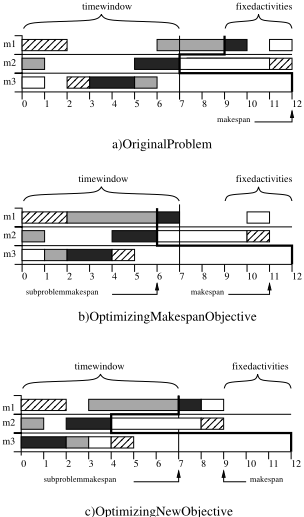
The time decomposition remains essentially a flexible shop problem, and can be solved using the same algorithms. However, since the problem is now decoupled, knowledge of how the re-optimized schedule will affect the overall solution is missing. Moreover, using the makespan minimization as objective is not flexible enough as we will illustrate shortly. It is more appropriate to use an objective function that maximizes the distance between each activity and their completion time bounds, allowing a better left shift of the entire schedule.
Definition (Time Decomposition Objective). The objective of a time decomposition 〈Rd , P d , α, β, γ, φ〉 is defined by
Figure 2 illustrates the benefit of this new objective. Part (a) shows the decomposition (jobs are denoted by colors), Part (b) shows the optimized schedule using the makespan objective, and Part (c) the schedule obtained with new objective. The new objective achieves a better makespan overall, although its local makespan is worse.
6.2 Machine Decomposition
The idea behind the machine decomposition is to extract a subproblem by selecting activities executing on a subset of the machines Md .
Definition. A machine decomposition 〈Rd , P d , md , α, β〉 of a solution (σo, μo) wrt a set Md of machines is a flexible shop defined over the activities Rd = {a ∈ A|μo(a) ∈ Md }, with precedence constraints P d = {(a, b) ∈ P|a ∈ Rd ∧b ∈ Rd }, with bounds on the activity starting times
and a reduced set of machines md (a) for all activities a ∈ Rd defined by md (a) = m(a) ∩Md . A feasible solution to a machine decomposition satisfies all constraints of the flexible shop, as well as the additional constraints:
Since the machine decomposition has full knowledge of the activities within each machine, minimizing the makespan guarantees the generation of non-degrading solutions as long as machines on the critical path are in the set Md .
6.3 SolutionMerging
Time and machine decompositions ensure that precedence and machine availability constraints are satisfied with respect to the original solution. As a result, it is possible to combine the machine assignments and the machine precedences to merge the solutions.
Definition. Let (σd, μd) be a solution from the time decomposition 〈Rd ,P d , α, β, γ, φ〉 wrt (σo, μo) and 〈s, e〉. The merging of (σd, μd) and (σo, μo) is the solution (σm, μm) obtained byμm(a) = μd(a) if a ∈ Rd μm(a) = μo(a) otherwise
and such that σm is assigned a start date minimizing the set of precedence constraints
The merging is similar for the machine decomposition.
7 Experimental Evaluation
The proposed algorithms were evaluated on the eData set of flexible shop instances from [Hurink et al., 1994]. Results are reported over the set of instances la21 to la40 which are the largest of the set (the remaining instances being relatively easy). The algoritms were implemented on top of the COMET system and run on an Intel 2.8 GHz Xeon processor with 8Gb of RAM. Due to the non-deterministic nature of the searches, average results over 10 runs are reported.
The large neighborhood algorithms LNS and the decomposition algorithm ARD using CP or LNS for subproblems were compared to the two best-performing heuristic algorithms. We use the following notations: TB stands for the tabu search of [Mastrolilli and Gambardella, 2000], hGA for the hybrid genetic algorithm of [Gao, 2008], hLNS for the LNS search using an hybrid random selection of the proposed relaxations, ARD(CP) for the ARD procedure using CP as a search algorithm and ARD(LNS) ARD using hLNS. Both ARD(CP) and ARD(LNS) use an adaptive selection for time windows in the following sense: if no improvement is found within 5 iterations, the size of decomposition increases, only to be brought back to the initial size upon finding an improved solution.
The ARD(CP) and ARD(LNS) use a time decomposition chosen between 20% and 50% of the horizon, with 5% step increase. The machine decomposition uses |M|/2 machines. The hLNS search selects activities with 50% probability in the random relaxation, time windows randomly chosen between 25% and 50% of horizon, and a number of machines randomly selected in [2, |M|/4] in the machine relaxation. Three additional relaxations are derived from these relaxations by fixing the machine of a relaxed activity to its current selection with a 33% probability.
Overall Quality of the Results Table 1 depicts the quality of solutions found in 5 and 10 minutes by using the Mean Relative Error (MRE) computed as 100%(UB - LB)/LB. The first column describes the set of instances, while the following columns present the aggregated results for each of the algorithms, giving the best performance and showing the average performance in parenthesis. Algorithms hLNS, ARD(CP), and ARD(LNS) achieve comparable results to those found using the best heuristic methods and the best solutions of hLNS and ARD(LNS) often produce improvements over the dedicated heuristics, in particular on la21-25 and la26-30. Note also that hLNS and ARD produces results that are about 0.5% in average from the best upper bound.
These results are surprisingly good, given that the CBS algorithms use a rather simple search: They thus require very little development effort on top of a modern constraint-based scheduler (e.g., LNS adds another 50 lines of code) and could certainly be improved by using more advanced search techniques, such as texture-based heuristics [Beck et al., 1997].
Table 2 presents the best results for runs of 5 and 60 minutes for all the experiments. Bold face means an improvement over the best known upper bound (last column) while italics means that the best known upper bound has been matched. It is interesting to point out that hLNS improves or matches all the best results in 60 minutes and improves more than 50% of them. In fact, hLNS produces similar results after 5 minutes, except on two benchmarks. ARD(LNS) produces relatively similar results: After a hour, it improves or matches all the best-known upper bounds except on two instances. The results after 5 minutes are a bit weaker but they still improve or match many of the best-known solutions.
| Problem | hLNS | ARD(CP) | ARD(LNS) | TB | hGA | |||
|---|---|---|---|---|---|---|---|---|
| 5 min | 10 min | 5 min | 10 min | 5 min | 10 min | |||
| la21-25 | 5.48 (6.13) | 5.48 (5.98) | 5.77 (6.73) | 5.57 (6.55) | 5.61 (6.50) | 5.59 (6.25) | 5.62 (5.93) | 5.60 (5.66) |
| la26-30 | 3.09 (4.41) | 2.95 (4.05) | 3.78 (4.89) | 3.33 (4.48) | 3.86 (5.13) | 3.16 (4.39) | 3.74 (3.76) | 3.28 (3.32) |
| la31-35 | 0.88 (1.25) | 0.46 (0.97) | 0.45 (1.08) | 0.32 (0.89) | 0.62 (1.33) | 0.32 (1.03) | 0.30 (0.32) | 0.32 (3.32) |
| la36-40 | 8.95 (10.09) | 8.91 (9.89) | 10.04 (11.52) | 9.48 (11.29) | 9.57 (10.95) | 9.44 (10.42) | 8.99 (9.13) | 8.82 (8.95) |
| Problem | ARD(CP) | ARD(LNS) | hLNS | UB | |||
|---|---|---|---|---|---|---|---|
| 5 min | 60 min | 5 min | 60 min | 5 min | 60 min | ||
| la21 | 1025 | 1016 | 1017 | 1015 | 1014 | 1009 | 1017 |
| la22 | 881 | 881 | 882 | 880 | 880 | 880 | 882 |
| la23 | 950 | 950 | 950 | 950 | 950 | 950 | 950 |
| la24 | 909 | 909 | 908 | 908 | 909 | 908 | 909 |
| la25 | 941 | 941 | 942 | 936 | 940 | 936 | 941 |
| la26 | 1124 | 1111 | 1127 | 1109 | 1110 | 1107 | 1125 |
| la27 | 1186 | 1182 | 1189 | 1182 | 1182 | 1181 | 1186 |
| la28 | 1149 | 1145 | 1147 | 1144 | 1148 | 1142 | 1149 |
| la29 | 1122 | 1117 | 1129 | 1111 | 1111 | 1111 | 1118 |
| la30 | 1219 | 1214 | 1212 | 1196 | 1211 | 1195 | 1204 |
| la31 | 1541 | 1533 | 1554 | 1541 | 1565 | 1539 | 1539 |
| la32 | 1698 | 1698 | 1698 | 1698 | 1698 | 1698 | 1698 |
| la33 | 1547 | 1547 | 1547 | 1547 | 1547 | 1547 | 1547 |
| la34 | 1609 | 1599 | 1609 | 1599 | 1618 | 1599 | 1599 |
| la35 | 1736 | 1736 | 1736 | 1736 | 1736 | 1736 | 1736 |
| la36 | 1174 | 1162 | 1167 | 1160 | 1160 | 1160 | 1162 |
| la37 | 1397 | 1397 | 1397 | 1397 | 1397 | 1397 | 1397 |
| la38 | 1156 | 1143 | 1159 | 1143 | 1148 | 1143 | 1144 |
| la39 | 1198 | 1186 | 1187 | 1184 | 1184 | 1184 | 1184 |
| la40 | 1167 | 1161 | 1157 | 1147 | 1146 | 1144 | 1150 |
Observe that hLNS explores larger neighborhoods than ARD(LNS) (since the relaxed activities can be inserted anywhere in the schedule), as well as the additional random neighborhood. It is thus not surprising that hLNS dominates ARD(LNS) on these instances. What is interesting is how close their performances are: This provides some preliminary evidence that ARD(LNS) may provide high-quality solutions quickly to large instances for which it would be too costly to reason about the schedule globally.
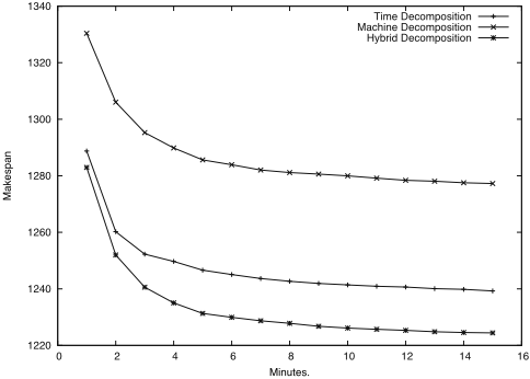
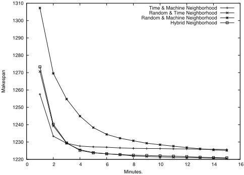
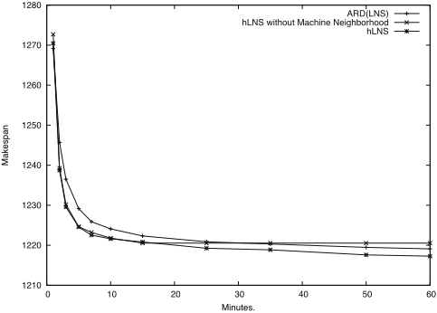
Impact fo the Neighborhoods We now study the impact of the various neighborhoods and decompositions on runs of 15 minutes. Figure 3 compares the time and machine decompositions, as well as their hybridization. The results show the clear benefit of the hybridization. Figure 4 depicts the results for large neighborhood search. For these runs of 15 minutes, they indicate that the random and time neighborhoods are most important: The machine neighborhood does not seem to bring additional benefits. Figure 5 shows that the machine neighborhood provides improvements for longer runs: It compares LNS with and without the machine neighborhood and ARD(LNS). The results indicate that the machine neighborhood starts improving the results after 15 minutes and is necessary for LNS to dominate ARD(LNS). These results also shed some interesting light on the strength of the decomposition approach, which does not rely on the random neighborhood, giving us some reasonable confidence that it will scale nicely on large-scale instances.
8 Conclusion
This paper presented large neighborhood and adaptive randomized decomposition approaches to the flexible jobshop problem. It demonstrated that a simple CBS formulation, enhanced with LNS or ARD, provides very high-quality results quickly on some standard classes of benchmarks and requires little development effort on top of a modern CBS systems. Moreover, the approaches improved 60% of the best upper bounds, while matching the remaining ones. The quality of the decomposition approach indicates that it is likely to scale to large-scale problems for which considering the problem in its entirety is not feasible. These results were achieved without advanced heuristics or learning techniques [Carchrae and Beck, 2009], suggesting that there is room for significant improvements. Overall, these results seem to confirm that LNS and ARD over a CBS formulation is an effective and generalpurpose approach to many complex scheduling problems.
@inproceedings{ijcai2011p333,
  title     = {Large Neighborhood Search and Adaptive Randomized Decompositions for Flexible Jobshop Scheduling},
  author    = {Pacino, Dario and Van Hentenryck, Pascal},
  booktitle = {Proceedings of the Twenty-Second International Joint Conference on
               Artificial Intelligence, {IJCAI-11}},
  publisher = {AAAI Press/International Joint Conferences on Artificial Intelligence},
  editor    = {Toby Walsh},
  pages     = {1997--2001},
  year      = {2011},
  month     = {7},
  doi       = {10.5591/978-1-57735-516-8/IJCAI11-333},
  url       = {https://doi.org/10.5591/978-1-57735-516-8/IJCAI11-333},
}
TY - CPAPER TI - Large Neighborhood Search and Adaptive Randomized Decompositions for Flexible Jobshop Scheduling AU - Pacino, Dario AU - Van Hentenryck, Pascal T2 - Proceedings of the Twenty-Second International Joint Conference on Artificial Intelligence, IJCAI-11 PB - AAAI Press/International Joint Conferences on Artificial Intelligence PY - 2011 SP - 1997 EP - 2001 DO - 10.5591/978-1-57735-516-8/IJCAI11-333 UR - https://doi.org/10.5591/978-1-57735-516-8/IJCAI11-333 ER -Copied
Machine-readable versions of this paper, for tools and AI agents:





