Modeling Multivariate Spatio-Temporal Remote Sensing Data with Large Gaps

1 Introduction

Applicability of many existing data analysis methods that assume fairly complete data is limited by the presence of a large fraction of missing values (gaps) in data. These gaps are often large among spatio-temporal observations by remote sensing instruments due to the presence of clouds, malfunctions of remote sensing instruments and noise. Although many sound statistical methods exist for imputation of missing values (e.g. multiple imputation [Rubin et al, 1987]) most of existing methods are not applicable when gaps in data are very large. To address large gaps in surveys, data mining alternatives were proposed that exploit similarity information from shared neighbors [Ayuyev et al, 2009].

In multivariate spatio-temporal data analysis problems of natural systems in the presence of large gaps three kinds of correlation could be potentially exploited. These opportunities consist of temporal correlation of attributes, correlations among multiple attributes collected at the same time and space, and spatial correlations among attributes collected at multiple sites. Although many methods were proposed that take advantage of one or two of these aspects, less work was devoted to taking into consideration all three kinds of correlations simultaneously. Exploiting these correlations to impute large gaps in multivariate spatio-temporal data to develop more accurate supervised prediction models is the objective of our study.

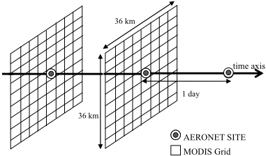
Our work is motivated by the multivariate spatio-temporal prediction task of large interest in geosciences called Aerosol Optical Depth (AOD) retrieval. AOD retrieval data is obtained by integrating remote sensing observations with large gaps from multiple sources and with multiple kinds of correlation among attributes. In this application 19 real value satellite-based attributes were derived from multi-spectral images obtained once per day for the entire Earth by MODIS instrument on Terra satellite [Modis, 2011]. We use such satellite data provided at a 4km*4km grid covering the entire continental US in year 2005 (illustrated for two days at Figure 1 for a 36km*36km region). Although MODIS provides daily coverage of almost entire Earth, all 19 attributes are missing at nodes corresponding to locations where it was cloudy at time of the satellite overpass and such events are very common. Real valued AOD outcome variable is measured from ground at a small number of AERONET locations [Aeronet, 2011]. Due to high cost of such ground-based data collection, in year 2005 only 33 AERONET sites were available in the entire continental US. The objective of AOD retrieval is to use spatio-temporally collocated MODIS attributes and AERONET outcomes to build an accurate AOD predictor that can estimate AOD value from satellite attributes. In this application one of the main challenges is a small number of spatio-temporally collocated MODIS observations and AERONET AOD outcomes. In particular, in year 2005 for the entire Continental US there were only 805 spatio-temporal events where both satellite and ground-based data were available. Using the method proposed in this article, This set is enlarged about five times to 4112 cases by imputing missing MODIS attributes by exploiting correlations among 19 attributes collected at a single node of the grid, spatial correlations of attributes observed at the same day at neighboring 80 nodes in 4x4km grid, and temporal correlations over multiple days. This allowed construction of much more accurate AOD retrievals as will be discussed in the results section.

The rest of the paper is organized as follows. The related work is briefly reviewed in Section 2. The proposed method for modeling multivariate spatio-temporal data is presented in Section 3 together with an algorithm for estimating missing observation. Evaluation results of the proposed method on both synthetic and real data sets are reported in Section 4. Section 5 provides the conclusion of our study.

2 Related Work

Many of the existing spatio-temporal data analysis methods assume that data is complete or almost complete. This assumption is violated in many spatio-temporal applications.

For estimation of missing values in multiple time series, a dynamic Bayesian model called DynaMMo was recently developed to simultaneously exploit temporal smoothness of each series and their correlations [Li et al, 2009]. Although very effective for estimating missing values in coevolving time series, DynaMMo is less applicable to remote sensing where data is collected at multiple spatially correlated locations where multiple correlated time series are observed at each location and individual series have temporal continuity.

For imputing incomplete spatial data, one of the most successful practical methods is to use multivariate interpolation by empirical orthogonal functions [Beckers et al, 2003]. In this singular value decomposition (SVD) based data imputation approach that we will simply call EOF, missing values are initially replaced by an unbiased guess and the missing values were interpolated incrementally by using truncated orthogonal functions of SVD decomposition for reconstruction and repeating the process while increasing the number of component functions. A limitation of EOF based data imputation is that it exploits only spatial correlations in data which is a problem when long continuous gaps are present in spatio-temporal data. An application of EOF to a transposed matrix that we will call T-EOF is proposed as a practical way to address such larger gaps in data [Kondrashov et al, 2006]. The same technique of using a transposed data to catch a different aspect of correlations in data (spatial instead of temporal) can also be applied to linear interpolation and to DynaMMo imputations. Such versions we will call T-Linear and T-DynaMMo methods.

Previous work [Radosavljevic et al 2010] in developing data-driven AOD retrieval methods using spatio-temporally collocated satellite and ground based observations (as shown at Figure 1) was simply removing the missing observations. The hypothesis explored in this study is that the accuracy of previously developed AOD predictors can be improved significantly by estimating the missing attributes and then train predictors on the data set consisting of both observed and imputed attributes.

3 Methodology

Given a multivariate spatio-temporal data (a multi-dimensional sequence and bunch of neighboring multi-dimensional sequences), there are three types of correlations: temporal correlation of each dimension, correlations among multiple dimensions collected at the same time and space, and spatial correlations from neighboring sites. Our goal is to build an accurate model on enlarged data with imputed values estimated by exploiting all three kinds of correlations.

3.1 Modeling correlations in a single sequence

In this section we describe how to model temporal correlation of each dimension and correlations among multiple dimensions from a multivariate sequence. We build a probabilistic model to estimate the missing values conditioned on observed values by exploiting these two types of correlation.

Assume that an m-dimensional sequence X = {x1, x2,É,xN} of length N is given, where vector xn observed at the n th time tick of sequence (n = 1,É,N) is a m-dimensional multivariate Gaussian. For each m-dimensional observation of vector xn we introduce a Gaussian latent variable zn such that there is a linear dependence with a Gaussian noise between each xn and zn defined as n n n x C , where C is the parameter matrix and is the Gaussian noise with mean of zero and variance of . z v ~ ( | 0, ) N v v

We also define a linear dependence with Gaussian noise between two adjacent latent variables zn-1 and zn corresponding to two successive observation xn-1 and xn as n n-1 z Az w n , where A is the parameter and is the Gaussian noise with mean of zero and variance of . ~ ( | 0, ) N w w

Therefore, the emission and transition distribution can be written as

The initial latent variable z1 also has a Gaussian distribution which can be written as

where 0 is the initial state of z1 and is the variance. 0 V

Let be the parameters of the model. Therefore, the joint probability given is { , , , , , } 0 0 A C V ( , | ) ( | , ) p p 1 0 0 X Z z V

Our model is different to the traditional Kalman Filter -based model, since we allow missing values to exist in the observation X. We define a Missing Index Matrix I to indicate the missing values. Each entry of is defined as I

For learning the model, we define the expectation of the complete-data log likelihood as

First, we initialize each missing value Xpq in data sequence (where ) using simple linear interpolation from the values where at the same time. Then, we apply the EM algorithm to maximize the equation (6). By extending the equation (6) by substituting using the corresponding part from equation (4) and (1)-(3), we get 0 pq I 0 pq I ( , | ) p X Z

where const is the term which is not dependent on any part of parameter .We take the derivatives of equation (7) with respect to each part of parameter and then set them to zero. We get the parameters updates as follows:

E

E

[B ]B B [

z z A

T

n-1 n-1

](

) }

E

n

[

n

]

E

[

n n

](

x z C C z z C

) }

At the end of each M step, we update the missing value Xpq (when ) using 0 pq I

Calculating the updated parameters requires the inference in E step of the marginal distribution for hidden latent variables given the data. The inference is similarly to ( | , ) p Z X

T new new

T

new T

T new new new T

the one in Kalman Filter-based model, since the missing values are updated at the end of each M step. We apply forward-backward message passing to calculate the expectation of posterior distribution of latent variables. The details of inference in the Kalman Filter-based model are omitted for lack of space (for more details see [Bishop et al, 2006]).

Then, we use the updated X to recalculate the new parameters in the next EM iteration. We repeat this procedure until convergence. The estimation for missing values can be automatically obtained once the model is learned.

3.2 Modeling spatial correlations from neighbors

In this section, we describe how to explore spatial correlations among neighboring sites. We build a probabilistic model among multivariate sequence X and its neighboring observations to estimate the missing values in X conditioned on the observed values in neighboring sites.

j Given a multivariate sequence X, let Li = {li1, li2,É,liN} (i = 1,Ém) be the i th dimension of X, where lin (n = 1,É,N) is a single value of the observation in the i th dimension at the n th time-step. Assuming that X has observations at k neighboring locations, we define as the i ( ) ( ) ( ) ( ) 1 2 { , ,..., } j j j i i i iN l l l L th dimension of XÕs j th (j = 1,É,k) neighboring locations. Our objective is to impute the missing value in each Li by exploiting the spatial correlation among Li and ( ) { | 1,..., } j i L j k } j . In order to learn such spatial correlation, for each dimension Li of X and corresponding from XÕs neighbors, we define as the union of L ( ) ( ) ( ) ( ) 1 2 { , , ..., j j j i i i iN L l l l (i) (i ) (i ) (i ) 1 2 N { , ,..., } O o o o i and ( ) { | 1,..., } j i j k L , where (n = 1,É,N) are the values of the i i (1) (2) { , , ,... } k n in in in in l l l l o ( ) th dimension of X and its neighboring locations at the n th time-step. For each observation , we define a Gaussian latent variable i n o ~ (0, ) N n y w } represents a ( ) i n o n} are

(n = 1,É,N). Each pair of nodes {yn, linear-Gaussian latent variable model for the particular multivariate observation. However, the latent variables {y treated as independent to each other. Hence, the emission distribution is

Then, we can build a probabilistic graphical model for each dimension of X to exploit the spatial correlation between each Li and its corresponding ( ) { | 1,..., } j i j k L from neighboring locations. Let { , , } w D be the parameters of the model. Then, the joint distribution can be written as:

Therefore, maximizing the complete data log likelihood is equivalent to maximizing:

We take the derivatives of equation (17) with respect to , D and w respectively, and set them to zero. The updated parameters are computed as

In order to get the optimal parameters maximizing equation (17) in the presence of missing observations, for each dimension of X we maintain another Missing Index Matrix where indicates a missing value of ( ) i I ( ) 0 i pq I ( ) i pq O . We initialize the each missing value using linear interpolation from values where in the neighboring observations. Then, we calculate new parameters using equation (18)-(20) ( ) 0 i pq I

and use them to estimate the missing values as

( ) ( ) ( ) ( ) ( ) { , } [ | , , ] [ | ] ( i i new i i pq new p q pq pq E E wh O Y I D Y O I 0) en (21) After imputing the missing values using eq. (21), we use the new data to estimate new parameters in the next iteration. By repeating this process of estimating parameters and missing values until converging, we can get the optimal parameters of the model and the final estimation of missing values. After updating the missing values in ( ) i pq O for each dimension of

X, we can get the estimated X.

3.3 Learning algorithm

In order to estimate the missing values by exploring all three types of correlation, we propose the LarGEST algorithm (shown in Algorithm 1) which simultaneously learns two models described in Sections 3.1 and 3.2.

First, we initialize all model parameters and fill all the missing values by linear interpolation from the values of spatial neighbors. Then, we apply an Extended Expectation Maximization algorithm which works as follows.

In the E-step, we estimate the posterior distribution ( | , ) p Z X of Model 1 which will be used when we maximize the expectation of log likelihood in M-step (using equations (8) -- (13)). After getting the updated parameters of Model 1, we can estimate the missing values using Model 1. The data with updated missing values from Model 1 is used to estimate the parameters of Model 2. We can re-estimate the missing values after learning the parameters of Model 2. The updated data with updated missing values estimated by Model 2 will be the input data of E-step of next iteration to calculate the posterior distribution of Model 1. We repeat this procedure of training two models interactively until convergence. Our experiments show that different order of two models has no significant influence in learning results since it only results in the different initialization values of two models.

After imputing the missing values in multivariate spatio-temporal data, we then build a predictor on enlarged collocated spatio-temporal data. In the next section we compare results of predictors trained on enlarged dataset generated by LarGEST and by alternative methods.

Inputs: X - set of multivariate spatio-temporal sequences with missing values { } - multivariate observations including ( ) i O neighbors for each dimension of X - Missing value Index Matrix for X I -Missing value Index Matrix for ( ) i I ( ) i O Outputs: X new Ð sequences with estimated values , Ð model parameters Initialize X new with X Estimate missing values in X new using linear interpolation Initialize model parameters Do E-step: Estimate posterior distribution of ( | , ) p Z X Model 1 using forward-backward message passing. M-step: Maximize expectation of log likelihood (Model 1) argmax ( ) new Q Estimate missing values using Model 1: for p, q DO update X new pq when Ipq=0 using equation (14) Initialize { } with X ( ) i new O new and { } ( ) i O Maximize log-likelihood (Model 2 for each dimension i): ( ) argmax ln ( , | ) new i new p O Y Estimate missing values using Model 2 for p, q DO update when I ( ) ( ) i pq new O pq=0 using eq. (21) X new = { } ( ) i new O Until converge Return X new , , and

4 Experimental Results

The proposed LarGEST method for imputation of large gaps in data is compared experimentally with Linear, DynaMMO and EOF methods. In addition, LarGEST is also compared to the same three methods when used on transposed data and such results are annotated as T-Linear, T-DynaMMo and T-EOF. Brief descriptions of six alternative methods are provided in Section 2.

Our evaluation is performed on three datasets of increasing complexity. In the first task (Section 4.1) the objective was to compare LarGEST to alternatives for imputing 5% to 90% missing values in a fairly simple function. In Section 4.2 this is followed by imputing 80% of missing values in a more challenging problem of Floride estimation whereas a similar data was used as a testbed in an earlier study [Li et al, 2009]. Finally, in Section 4.3 effects of data imputation by LarGEST and alternatives were compared at a grant challenge problem of spatio-temporal regression for Aerosol AOD retrieval from data with about 80% of missing values in 19 attributes.

4.1 Imputation of small versus large gaps

The synthetic two dimensional temporal data (X, Y) for a certain location is generated as sin( )*5 X t and sin( / 2)*5 Y t . At four neighboring locations two dimensional data is generated by shifting the first site data by 0.5 0.3, -0.3and -0.5 respectively.

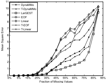
The mean square error (MSE) of imputation by LarGEST and six alternatives was compared when 5% to 90% of data were missing randomly (see Figure 2). In data imputation experiments with small fraction (less than 25%) of missing values inserted completely at random, LarGEST and all alternative methods estimated missing values fairly well. However, LarGEST was clearly the best choice as Linear interpolation had problems when the missing values were located near the top or the bottom of the signal, while EOF had problems where four neighbors were missing and DynaMMo had some errors at high curvature sections.

Fraction of Missing Values

Figure . Estimated error (MSE) for imputing 5% to 90% of missing values on synthetic data.

When large fraction of data was missing LarGEST exploited well all three kinds of correlations in data simultaneously while alternative imputation methods resulted in much larger error. When extremely large fraction (85% and 90%) of data was missing, all methods performed badly. For a large fraction of missing values accuracy was improved when the number of neighbors was increased. Results with a larger number of neighbors are omitted on synthetic data for lack of space, but will be shown on real remote sensing data.

4.2 Imputation of 80% gaps in Fluoride data

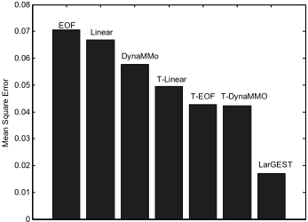
The Fluoride dataset is produced by EPANET 2 which models the water quality behavior in a distribution piping systems. In a given network of water distribution piping system, EPANET simulates the contents of Fluoride over a certain period [EPA, 2011]. Data used in our experiments are generated assuming a piping system of 36 nodes simulated over 10 days in 15 minutes increments. For our experiments at a certain node and at its three neighboring nodes we extracted two attributes over 960 time steps. Then, 80% of this data was removed completely at random from each of two attributes at each of 4 nodes retaining 192 values per each attribute at each site. The objective was to estimate 1536 missing values at two time series observed at one of these nodes. The mean square error (MSE) of this estimation by LarGEST and alternative methods are shown at Figure 3.

4.3 Spatio-temporal regression of Aerosol data with 80% of imputed attributes

Experiments were conducted on integrated satellite and ground based Aerosol data introduced in Section 1. AOD

0

Figure 3. Mean square error of data imputation on Fluoride data with 80% of missing values.

values observed from ground at 33 AERONET sites were also available at an additional 3,307 events, but in these cases all 19 sattelite-based attributes were missing. Missing attributes at these 80% cases were imputed by LarGEST relaying on spatial correlations with satellite observations at up to 80 neighbors at 4kmx4km grid as well as on temporal correlations among 330 daily observations. Six alternative methods used in Section 4.1 were also applied for attributes imputation at 3,307 events.

A feed-forward neural network model with a single hidden layer of 10 nodes was trained on enlarged data consisting of examples with actual and those with imputed attributes. This choice was based on the best predictors from previous studies [Radosavljevic. et al, 2010]. Experiments were performed by partitioning 805 examples from 33 sites where both attributes and AOD values are available in 33 disjoint subsets based on sites and using 32 subsets together with 3,307 additional examples whose attributes are imputed for training a neural network model which is tested on the remaining siteÕs data. This is repeated in 33-cross validation experiments always keeping a different site for testing. The quality of the obtained predictors was compared using two measures following a protocol practiced by geoscience community [Radosavljevic et al, 2010]. To evaluate impact of spatial neighborhood size on imputation quality, in LarGEST imputation we considering nearest 8, 24, 48 and 80 neighboring observations in 4kmx4km grid shown at Figure 1. These methods we will call LarGEST8, LarGEST24, LarGEST48 and LarGEST80, respectively.

Learning time is not a concern in this application. In 10 minutes our method imputes data streams used in our experiments on a desktop computer with only 3 GB memory. This time is negligible as compared to months of simulations on a supercomputer required by traditional deterministic aerosol retrieval methods based on physical modeling.

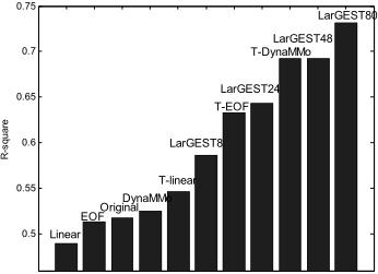
The first quality measure we used is R-square. The results obtained by a predictor trained on data imputed by LarGEST80, and by nine alternative methods are shown in Figure 4. In addition, we also show the accuracy of a predictor obtained on 805 examples without data imputation and we call this model Original. The results obtained by LarGEST80 were more accurate than alternatives and better than any previously reported accuracy of AOD retrieval.

0.66

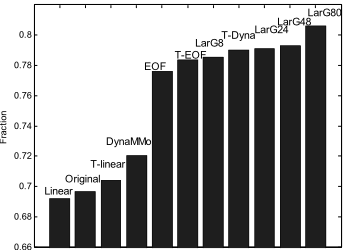
Figure 5. Fraction of successful AOD retrievals in US for year 2005 when using 80% imputed values (LarG in the figure means LarGEST )

Another measure we used is introduced by aerosol scientists who regard the retrieved AOD acceptable if the following boundary conditions on the retrieval are satisfied i where y | | 0.05 0.15 i i y t t i is retrieved AOD value and ti is the corresponding true AOD value. We measured fraction of successful predictions defined as , where I is the number of predictions satisfying the stated boundary and N is the total number of predictions. Fraction of successful AOD retrievals of seven regression models based on data imputed by LarGEST and six alternatives as well as data that is not imputed at all (called Original) are shown at Figure 5. LarGEST80 clearly outperformed all alternative methods in both measures. ( / )*100% FRAC I N

Both Figure 4 and Figure 5 show that LarGEST performed better when including attributes from larger number of neighboring grids. All 80 neighbors used in LarGEST80 model were within the range of 36km (see Figure 1) which is considered to be a range of AOD spatial correlation. Indeed, including spatial information from even more distant nodes was not beneficial (results omitted for the lack of space).

5 Conclusion

In the proposed method, two probabilistic models were proposed, and learned interactively by an Extended Expectation Maximization algorithm to exploit simultaneously all three types of correlation for multivariate spatio-temporal data imputation. The imputation results on challenging problems with 80% of missing values provide evidence that in the presence of long continuous gaps LarGEST method can estimate missing values more accurately than alternatives. The aerosol optical depth retrieval results obtained using training data enlarged by LarGEST-based imputations were not only better than the results obtained by training a predictor trained on data imputed using alternative methods, but were also more accurate than any previously developed method for AOD retrieval from satellite data.

Acknowledgments

This work was supported in part by the National Science Foundation under Grant IIS-0612149.