
Pattern Field Classification with Style Normalized Transformation
Proceedings of the Twenty-Second International Joint Conference on Artificial Intelligence. Pages 1621-1625.
https://doi.org/10.5591/978-1-57735-516-8/IJCAI11-272
© 2011 International Joint Conferences on Artificial Intelligence
Abstract
Field classification is an extension of the traditional classification framework, by breaking the i.i.d. assumption. In field classification, patterns occur as groups (fields) of homogeneous styles. By utilizing style consistency, classifying groups of patterns is often more accurate than classifying single patterns. In this paper, we extend the Bayes decision theory, and develop the Field Bayesian Model (FBM) to deal with field classification. Specifically, we propose to learn a Style Normalized Transformation (SNT) for each field. Via the SNTs, the data of different fields are transformed to a uniform style space (i.i.d. space). The proposed model is a general and systematic framework, under which many probabilistic models can be easily extended for field classification. To transfer the model to unseen styles, we propose a transductive model called Transfer Bayesian Rule (TBR) based on self-training. We conducted extensive experiments on face, speech and a large-scale handwriting dataset, and got significant error rate reduction compared to the state-of-the-art methods.
- [Caruana, 1997] Rich Caruana. Multitask learning. Machine Learning, 1997.
- [Gourier et al., 2004] N. Gourier, D. Hall, and J. Crowley. Estimat- ing face orientation from robust detection of salient facial fea- tures. In ICPR, 2004.
- [Hastie and Tibshirani, 1996] T. Hastie and R. Tibshirani. Discrim- inant adaptive nearest neighbor classification. IEEE Trans. PAMI, 1996.
- [Kimura et al., 1987] F. Kimura, K. Takashina, S. Tsuruoka, and Y. Miyake. Modified quadratic discriminant functions and the application to Chinese character recognition. IEEE Trans. PAMI, 1987.
- [Liu and Zhou, 2006] C.-L. Liu and X.-D. Zhou. Online Japanese character recognition using trajectory-based normalization and direction feature extraction. In IWFHR, 2006.
- [Liu et al., 2011] C.-L. Liu, F. Yin, D.-H. Wang, and Q.-F. Wang. CASIA online and offline Chinese handwriting databases. In IC- DAR (submitted), 2011.
- [Pan and Yang, 2010] S.J. Pan and Q. Yang. A survey on transfer learning. IEEE Trans. KDE, 2010.
- [Sarkar and Nagy, 2005] P. Sarkar and G. Nagy. Style consistent classification of isogenous patterns. IEEE Trans. PAMI, 2005.
- [Tenenbaum and Freeman, 2000] J.B. Tenenbaum and W.T. Free- man. Separating style and content with bilinear models. Neural Computation, 2000.
- [Veeramachaneni and Nagy, 2005] S. Veeramachaneni and G. Nagy. Style context with second-order statistics. IEEE Trans. PAMI, 2005.
- [Veeramachaneni and Nagy, 2007] S. Veeramachaneni and G. Nagy. Analytical results on style-constrained bayesian classification of pattern fields. IEEE Trans. PAMI, 2007.
- [Zhang and Liu, 2011] X.-Y. Zhang and C.-L. Liu. Style transfer matrix learning for writer adaptation. In CVPR (to appear), 2011.
References were extracted automatically from the PDF and may contain errors.
Full text extracted automatically from the PDF; figures, tables and equations may differ. The PDF is the version of record.
1 Introduction
Statistical pattern recognition usually assumes that the patterns are independently and identically distributed (i.i.d.). However, in practical environments, patterns often occur as homogeneous groups (fields) generated by the same source. Moreover, the style of each group is consistent, implying statistical dependencies among patterns.
1.1 Field Classification
For a classification problem with feature space x ∈ Rd , and label space y ∈ {1, · · · ,M} (M is the number of classes), we have the following definition:
Definition 1 Denote a group of patterns and the corresponding labels as
If all the patterns in fi come from the same source with a consistent style, we call fi a field-pattern with field-length ni , and ci is the field-class. Note that when ni = 1, the field reduces to a singlet.
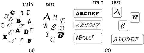
The patterns in a field are assumed to come from a common source. For example, in handwriting recognition, a fieldpattern is a group of characters produced by a certain writer with his/her individual writing style; in face recognition, face images can appear as different groups according to different poses or illumination conditions; in speech recognition, different speakers have different accents. These situations provide important group (field) information. The definition of field breaks the traditional i.i.d. assumption:
- Within each field, the patterns are NOT independent.
- Different fields are NOT identically distributed.
As the style in a single field is consistent, different fields usually have great style variations. The purpose of field classification is to train a classifier on the labeled field-patterns {fi, ci}Ni=1 (N is the number of training fields) for predicting the field-class of a new field-pattern (assigning labels for a group of patterns simultaneously). Note that a new fieldpattern unnecessarily enjoys the same style as the training field-patterns, which means style transfer exists between the training and test fields. This makes the problem even more challenging.
In the traditional i.i.d. based classification framework, the patterns are classified one at a time (Figure 1(a)), known as singlet classification. On the contrary, in field classification, a group of patterns are classified simultaneously (Figure 1(b)). By utilizing style consistency in each field, field classification will give higher accuracy than singlet classification.
1.2 Previous Work
Despite its importance, the field classification problem has been rarely studied in the literature. [Sarkar and Nagy, 2005] proposed a style mixture model which assumes a fixed number (say K) of styles across all the patterns. Under each style, the patterns are i.i.d. The distribution of a field-pattern is a mixture of the K styles. On one hand, the style number needs to be fixed before hand; on the other hand, for a newly coming field-pattern of different style from the K styles, this model does not promise good performance. Another related model was proposed by assuming Gaussian field-class-conditional distribution [Veeramachaneni and Nagy, 2005]. However, the model is merely valid for the Gaussian distribution, and its performance is rather limited due to its computational inefficiency. [Tenenbaum and Freeman, 2000] proposed a bilinear model to separate the style and content (class) information of patterns. However, this model can only predict labels for a field. When the patterns are coming one at a time (singlet), the model becomes unavailable. In addition, the optimization of this model requires the SVD decomposition of an Nd×M matrix, which is computationally inefficient when the number of classes M or the number of fields N is large.
1.3 Our Model
In contrast to previous works, in this paper, we extend the Bayes decision theory under two reasonable assumptions and develop the Field Bayesian Model (FBM) to deal with field classification. More specifically, we propose to learn a Style Normalized Transformation (SNT) for each field. Via the SNTs, the data of different fields are transformed to a uniform style space (i.i.d. space), where the traditional Bayesian classification model can apply. Our model is a general framework. Under this framework, we have shown how a multivariate Gaussian density model can be modified for field classification and achieve surprisingly good performance. Interestingly, the bilinear model for separating style and content [Tenenbaum and Freeman, 2000] is very similar to a special case under our framework. We have developed a lot of decision rules for classification on a newly coming single pattern or a field-pattern even if it shares no common styles with the training field-patterns (style transfer). We conducted extensive experiments on face and speech data as well as a largescale handwriting dataset (with 3, 755 classes and around 495K patterns). The experimental results are highly encouraging: we got significant error rate reduction compared to the state-of-the-art methods.
1.4 Related Topic
We note that field classification is also related to Multiple Task Learning (MTL) [Caruana, 1997] and Transfer Learning (TL) [Pan and Yang, 2010]. However, key differences exist in that our field classification model merely learns a single classifier, while MTL learns multiple classifiers (one for each task). In addition, while concept transfer is the main focus in TL, our proposed model cares about the same concept but with style transfer. Field classification is also closely related to classifier adaptation, where we should adapt the classifier from a style-independent domain to a style-specific domain [Zhang and Liu, 2011].
2 Field Bayesian Classification
The main idea of applying the Bayes decision theory to field classification is to assign the field-pattern to the field-class of maximum a posteriori (MAP) probability, which can be computed by the Bayes formula:
Here we omit the field index i and use f and c to represent a general field-pattern and field-class. The key problem is to define the field-class prior probabilities p(c) and fieldclass-conditional probability distributions p(f|c). Based on two reasonable assumptions as follows, we derive the Field Bayesian Model (FBM), develop the optimization algorithm, and provide special cases for practical purpose.
2.1 Basic Assumptions
The consistency of style in each field is known as style context [Veeramachaneni and Nagy, 2007], which is different from the linguistic and spatial context. To make full use of the style context, we have the following assumptions.
Assumption 1
We assume no higher order linguistic dependence than the prior class probabilities. This means we only care about the style context in each field. Linguistic contexts such as morphological and lexical context (already widely used in optical character recognition and automated speech recognition) are not our focus, but are usable in field classification if needed.
Since the number of field-class grows exponentially with the basic class number (for an M-class problem with fieldlength n, there are totally M n field-classes), we cannot define a distribution for each field-class. In light of this, we make the following assumption.
Assumption 2
Here we assume that under certain field-specific classindependent transformation gi(x), the patterns in each field become class-conditionally independent. This means after the transformation, the data of different fields are transferred to a uniform style space, where all the patterns are i.i.d. We call this process Style Normalized Transformation (SNT). A consequence of this assumption is the order independence, implying that under any permutation of the order of patterns in a field, the joint conditional probability is not changed. In other words, we only care about the style context in each field, while the spatial context like feature dependence between adjacent patterns, which could be captured by HMM and other models, is not our focus.
2.2 MainWork
From Assumption 2, we only need to define the single-class conditional probability distributions p(x|y) and the Style Normalized Transformation gi(x) for each field. In this paper, we assume the SNT to be an affine transformation (covering rotation, scaling, shear and shift transformations) gi(x) = A⊤i x + bi, where Ai ∈ Rd×d , bi ∈ Rd are the parameters.
Model Definition
Given labeled field-patterns {fi, ci}Ni=1 , we learn the singleclass conditional probability distributions p(x|y) and the field-specific SNT {Ai, bi}Ni=1 simultaneously. The likelihood function of the training data is
The parameters are estimated such that the likelihood function is maximized. Equivalently, the negative log-likelihood is minimized:
Directly minimizing NLL will lead to over-fitting. To alleviate this, we adopt a regularization term on the SNTs.
Problem 1 Field BayesianModel (FBM)
where the regularization term is
Here I is the d × d identity matrix. The first term of R is to constrain the deviation of A from the identity matrix, and the second term is to constrain the deviation of b from the zero vector. Setting β = γ = +∞ will lead to Ai = I, bi = 0, ∀i, implying no style variation. Hence, the FBM model seeks a balance between style transfer and non-transfer, which will give better generalization performance. Under the fieldspecific style normalized transformation (SNT), we can learn the style-invariant Bayesian model which is more relevant to the classification content. That means we separate the style and the content by the SNT and underlying Bayesian model.
Prediction on Future Patterns
Before we dive into solving the above optimization problem of FBM (7), we first introduce how to use the model to predict the labels of single patterns and field-patterns. We assume equal a priori probabilities as usually.
Classification for Singlet
We can use the traditional Bayes Decision Rule (BDR):
In order to make use of the SNTs (on training field-patterns) learned before, we propose a Voted Decision Rule (VDR):
This is the classification rule based on feature space perturbation.
Classification for Field
Different from the traditional singlet classification, field classification is to assign labels to a group of patterns drawn from the same source (a new field). If we already know the SNT parameters {A0, b0} of this field, e.g., we know exactly that the new field has the same style with one of the training fields, the patterns in the field can be classified one at a time by
we call this Field Decision Rule (FDR).
If the newly coming field-pattern f = {x1, · · · , xn} has an unseen style, we should predict the field-class c = {y1, · · · , yn} and simultaneously estimate the SNT parameters {A, b} via minimizing the negative log-likelihood:
We also adopt the same regularization as described above to avoid over-transfer. In short, the classification task can be formulated as a learning problem as follows.
Problem 2 Transfer Bayesian Rule (TBR)
This is a transductive model, where we transfer the Bayesian model to the new style via SNT {A, b}, and simultaneously deduce the labels {y1, · · · , yn}. Note we can still apply TBR after FDR (FDR+TBR), which means TBR is used to the transformed samples (A⊤0 x + b0). This is to learn an additional SNT, which can capture the style change over times.
Optimization
We solve the FBM and TBR problems using the alternating optimization algorithm, which gives a straightforward interpretation of our models.
For optimizing the FBM (7), the class-conditional distributions (classifier parameters) estimation and the SNT parameters estimation are alternated iteratively. When we fix the SNT parameters {Ai, bi}, it becomes the problem of parameter estimation of a traditional Bayesian model; when we fix the class-conditional distributions p(x|y), the problem can be decomposed into N independent optimization problems:
Problem 3 Style Normalized Transformation Learning
Here we omit the field index i. The SNT learning is applied for all the training fields.
For optimizing the TBR (13), the field-class deduction and the SNT parameters estimation are alternated iteratively. When we fix the SNT parameters {A, b}, it becomes the problem of classifying n patterns independently by the FDR rule; when we fix the labels {y1, · · · , yn}, the problem is to learn an SNT, which is the same as (14). The alternating optimization in this situation can also be viewed as self-training, since each step of parameters updating is based on the labels deduced in the previous step.
Remarks. The key problem is to solve the SNT model (14). After we solve (14), we can use the alternating optimization as described above to solve the FBM (7) or TBR (13). When the optimization problem is jointly convex with all the parameters (as observed in the special case in Section 2.3), the alternating optimization is guaranteed to find the global solution. In the non-convex situation, we can still find a good-enough local minimum via the alternating optimization. A suitable initialization can be made as Ai = I, bi = 0, ∀i for FBM and A = I, b = 0 for TBR.
2.3 Special Cases
While our framework can be easily applied to other probabilistic models, in this section, we focus on the behavior of FBM and TBR under the multivariate Gaussian classconditional probability distribution
where θk = {μk ∈ Rd ,Σk ∈ Rd×d } denotes the set of parameters for class k (k = 1, · · · ,M).
Now the SNT problem (14) becomes:
where dm(x, μ,Σ) = (x - μ)⊤Σ-1 (x - μ) is the Mahalanobis distance. This is a convex quadratic programming (QP) problem which has a closed-form solution. However, to solve this model, we should compute the inverse of a d2 × d2 matrix, which is intractable when d is large. Moreover, it is also practically difficult to achieve a precise estimation of the covariance matrix. Therefore, we consider two special cases.
The first one is based on the assumption that Σk = I, k = 1, · · · ,M. This leads to the Nearest Class Mean (NCM) classifier in the traditional Bayesian framework. Now (16) becomes:
This is a convex QP problem. Moreover, in this setting the FBM (7) problem is also a convex QP, implying that the alternating optimization algorithm described in Section 2.2 is guaranteed to find the global optimum. We call this model Field Nearest Class Mean (field-NCM). This model is closely related to the bilinear model used to separate style and content [Tenenbaum and Freeman, 2000], with the difference that our model is convex and we adopt a regularization term to avoid over-transfer.
We also consider another special case based on the K-L transformation of the covariance matrix [Kimura et al., 1987].
where Λ = diag[λ1, · · · , λd] with λt, t = 1, · · · , d, being the eigenvalues (ordered in non-increasing order) of Σ, and Φ = [φ1, · · · , φd] with φt, t = 1, · · · , d, being the corresponding eigenvectors. In most cases, the estimation of the minor eigenvalues are affected by noises or lack of samples. Therefor we only keep the largest T eigenvalues (T < d). Under this situation, we can change the Mahalanobis distance used in (16) to the projection distance by computing the Euclidean distance between the original point and its projection on the principal axes. The projection of point x onto the T principal axes of Σ is
where
We adopt a hyper-parameter δ ≥ 0 to constrain the deviation of the projection point from the class-mean (when δ = 0, P(x, Σ, μ) = μ).
Therefore, we can approximate (16) by:
Since under this situation, the classification boundary is quadratic, we call this model Field Quadratic Discriminant Function (field-QDF).
The SNT learning problems of the field-NCM (17) and the field-QDF (21) are both convex QPs, which take the general form as follows:
where sj = μyj for (17) and sj = P(xj,Σyj , μyj ) for (21). This problem has a closed-form solution:
where
The hyper-parameter β, γ acts as a tradeoff between style transfer and non-transfer. Considering the influence of data scaling, we set them as:
Where ˜ β and ˜ γ can be selected from [0,3] effectively via cross-validation or other methods.
3 Experiments
We conducted a series of experiments on three benchmark datasets (face, speech and handwriting).
The first purpose is to compare singlet classification (the patterns are classified one at a time) with field classification (a group of patterns with the same style are classified simultaneously). We choose the best decision rule for each case: BDR (9) and VDR (10) for singlet classification; FDR (11), TBR (13), and FDR+TBR for field classification. Note that the FDR assumes the test field has the same style with one of the training fields and the corresponding training field is known, and therefore, we used it only on the multi-writer handwriting dataset.
The second purpose is to compare field Bayesian models with: (1) two field models: the style mixture model [Sarkar and Nagy, 2005] and the bilinear model [Tenenbaum and Freeman, 2000]; (2) traditional state-of-the-art methods in three distinct domains. In order to make a fair comparison, the distribution of each mixture component in the style mixture model is assumed to be the Gaussian distribution with identity covariance matrix. The EM algorithm used in the bilinear model is initialized by the nearest class mean classifier.
3.1 Face Recognition under Different Poses
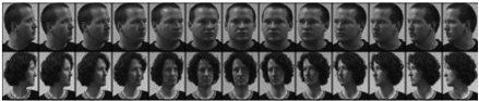
The pose database [Gourier et al., 2004] consists of the images of 15 persons. For each person with zero vertical pose angle, we used 13 horizontal pose angles varying from -90 to 90 degree (interval 15 degree) in our experiment, in total 195 face images. All the images are resized to be 48 × 36 pixels. The dimensionality is hence equal to 1728. We show the face images of two persons in Figure 2. Considering the 15 images of each pose as a field, we used the images of the 1-8 poses (the 1-8 columns) as training data, and tested on the remaining images (9-13 columns).
| NCM | Style Mixture | Bilinear | field-NCM | |
|---|---|---|---|---|
| Singlet | 40.00% | 30.00% | - | 25.33% (VDR) |
| Field | 40.00% | 26.67% | 40.00% | 21.33% (TBR) |
For a benchmark comparison, we first implemented the Fisherface model (FDA with subspace dimensionality 14), which gave the error rate 30.67% by the nearest class mean (NCM) classifier. To speed up computation for other methods, we reduced the dimensionality of images to 100 by PCA. The results are shown in Table 1. Due to a fixed number of mixture components, the style mixture model cannot transfer to new styles very well. The bilinear model cannot be applied for singlet classification. Moreover, the performance is deteriorated because the field-length was too small (there were only 15 images for each pose). However, our field-NCMwith TBR can still give the best result, because a regularization term is adopted to avoid over-transfer.
3.2 Multi-speaker Vowel Classification
We used a benchmark speech dataset 1 . This dataset consists of 11 vowels uttered by 15 speakers of British English, and there are six samples per speaker per vowel. Each sample vector consists of 10 log-area parameters, a standard vocal tract representation computed from a linear predictive coding analysis of the digitized speech. We follow the same setting used in [Tenenbaum and Freeman, 2000] and used the data of the 1-8 (9-15) speakers as the training set (test set). Each speaker is considered as a field which has a specific accent.
| Classifier | Error rate |
|---|---|
| Multilayer perceptron | 49% |
| Radial basis function network | 47% |
| 1-nearest neighbor | 44% |
| Discriminant adaptive nearest neighbor | 38.3% |
| NCM | Style Mixture | Bilinear | field-NCM | |
|---|---|---|---|---|
| Singlet | 49.35% | 46.11% | - | 39.39% (BDR) |
| Field | 49.35% | 44.15% | 22.70% | 21.65% (TBR) |
The results are reported in Table 2. As observed, without style modeling, the best result is obtained by the discriminant adaptive nearest neighbor (DANN) classifier [Hastie and Tibshirani, 1996]. For singlet classification, the field-NCMwith BDR performs comparably with the DANN classifier. Moreover, for field classification, the field-NCM with TBR gave 21.65% error rate, which is better than the best result of the bilinear model reported by [Tenenbaum and Freeman, 2000].
3.3 Multi-writer Handwriting Recognition
In this section, we consider a large-scale (3, 755 classes) online Chinese character recognition problem. We used the CASIA-OLHWDB [Liu et al., 2011] to evaluate our models. Specifically, we used the samples of 100 writers (no.1101 - 1200) from the database. For each writer, there are about 3, 755 isolated characters (which we used as the training set), and about 1, 200 characters extracted from handwritten texts (which we used as the test set). Hence, the total number of patterns is over 495K (375K for training and 120K for test). Because persons tend to write texts more cursively than isolated characters, the test data (samples from handwritten texts) show significant style transfer from the training data (isolated characters).
For representing a character sample, we used a benchmark feature extraction method [Liu and Zhou, 2006]: 8-direction histogram feature extraction combined with pseudo 2D bimoment normalization. The feature dimensionality is 512
1 The data were collected by David Deterding and are now available at http://archive.ics.uci.edu/ml.
which is further reduced to 160 by FDA. Each writer is considered as a field.
| NCM | Style Mixture | field-NCM | |
|---|---|---|---|
| Singlet | 18.18% | 19.88% | 16.07% (VDR) |
| Field | 18.18% | 17.93% | 12.90% (FDR+TBR) |
| field-QDF | ||||
|---|---|---|---|---|
| MQDF | VDR | FDR | TBR | FDR+TBR |
| 12.17% | 11.31% | 10.24% | 9.91% | 8.89% |
︸
︷︷
︸
Singlet Classification
︷︷
F ield Classif ication
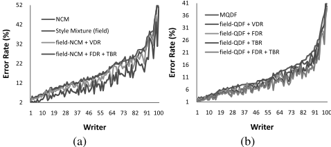
Figure 3: Error rates of different methods on the 100 writers, which are sorted in the increasing order of (a) the NCM error rates, (b) the MQDF error rates.
We did not report the performance of the bilinear model [Tenenbaum and Freeman, 2000] here because it is extremely time-consuming on the large-scale dataset. We report in Table 3 the average error rates of the traditional nearest class mean (NCM) classifier, the style mixture model and our field-NCM, while the error rates for each of the 100 writers are plotted in Figure 3(a). It is seen that the field-NCM combined with VDR achieves the best result for singlet classification. Moreover, the field-NCM combined with FDR+TBR gives the best result for field classification. It is noteworthy that the field-NCM combined with FDR+TBR performs always better than the other methods on all the 100 writers. This again shows the superiority of our proposed model.
The proposed field Bayesian model is a general framework, which can be combined with many probabilistic models. We also compared our field-QDF model with the state-of-theart classifier MQDF (modified quadratic discriminant function) [Kimura et al., 1987] in Chinese character recognition. The average results and specific results for each writer are shown in Table 4 and Figure 3(b). We can see that for singlet classification, the field-QDF with VDR outperforms the MQDF; and for field classification, the error rates of FDR, TBR and FDR+TBR decrease gradually, by learning the style information with increasing attention.
4 Conclusion and FutureWork
In this paper, we consider the field classification problem, where the patterns appear as groups of homogeneous styles.
︸
︸
To make full use of the style context in each field, we propose to learn a Style Normalized Transformation (SNT) for each field. With the SNTs, the data of different fields are transformed into an i.i.d. space, where the traditional Bayesian model can be applied effectively. In order to transfer the learned model to an unseen style, we propose the Transfer Bayesian Rule (TBR), which is a transductive model based on self-training, to predict the labels and the SNT parameters simultaneously from the test data. Experiments on three benchmark databases (face, speech and handwriting) demonstrated that our field models can reduce the error rates significantly compared with the other state-of-the-art classifiers. Our future work involves the extension to more complex class-conditional distributions other than the Gaussian distribution and the exploration of field classification using nonprobabilistic classifiers such as the SVM.
Acknowledgements
This work was supported by the National Natural Science Foundation of China (NSFC) under grants No. 60825301, No. 60933010 and No. 61075052.
@inproceedings{ijcai2011p272,
  title     = {Pattern Field Classification with Style Normalized Transformation},
  author    = {Zhang, Xu-Yao and Huang, Kaizhu and Liu, Cheng-Lin},
  booktitle = {Proceedings of the Twenty-Second International Joint Conference on
               Artificial Intelligence, {IJCAI-11}},
  publisher = {AAAI Press/International Joint Conferences on Artificial Intelligence},
  editor    = {Toby Walsh},
  pages     = {1621--1625},
  year      = {2011},
  month     = {7},
  doi       = {10.5591/978-1-57735-516-8/IJCAI11-272},
  url       = {https://doi.org/10.5591/978-1-57735-516-8/IJCAI11-272},
}
TY - CPAPER TI - Pattern Field Classification with Style Normalized Transformation AU - Zhang, Xu-Yao AU - Huang, Kaizhu AU - Liu, Cheng-Lin T2 - Proceedings of the Twenty-Second International Joint Conference on Artificial Intelligence, IJCAI-11 PB - AAAI Press/International Joint Conferences on Artificial Intelligence PY - 2011 SP - 1621 EP - 1625 DO - 10.5591/978-1-57735-516-8/IJCAI11-272 UR - https://doi.org/10.5591/978-1-57735-516-8/IJCAI11-272 ER -Copied
Machine-readable versions of this paper, for tools and AI agents:





