
LIFT: Multi-Label Learning with Label-Specific Features
Proceedings of the Twenty-Second International Joint Conference on Artificial Intelligence. Pages 1609-1613.
https://doi.org/10.5591/978-1-57735-516-8/IJCAI11-270
© 2011 International Joint Conferences on Artificial Intelligence
Abstract
Multi-label learning deals with the problem where each training example is represented by a single instance while associated with a set of class labels. For an unseen example, existing approaches choose to determine the membership of each possible class label to it based on identical feature set, i.e. the very instance representation of the unseen example is employed in the discrimination processes of all labels. However, this commonly-used strategy might be suboptimal as different class labels usually carry specific characteristics of their own, and it could be beneficial to exploit different feature sets for the discrimination of different labels. Based on the above reflection, we propose a new strategy to multi-label learning by leveraging label-specific features, where a simple yet effective algorithm named LIFT is presented. Briefly, LIFT constructs features specific to each label by conducting clustering analysis on its positive and negative instances, and then performs training and testing by querying the clustering results. Extensive experiments across sixteen diversified data sets clearly validate the superiority of LIFT against other well-established multi-label learning algorithms.
- [Boutell et al., 2004] M. R. Boutell, J. Luo, X. Shen, and C. M. Brown. Learning multi-label scene classification. Pattern Recognition, 37(9):1757-1771, 2004.
- [Chang and Lin, 2001] C.-C. Chang and C.-J. Lin. LIBSVM: A library for support vector machines, 2001. Software available at http://www.csie.ntu.edu.tw/˜cjlin/libsvm. Link
- [Cheng and Hüllermeier, 2009] W. Cheng and E. Hüllermeier. Combining instance-based learning and logistic regression for multilabel classification. Machine Learning, 76(2-3):211-225, 2009.
- [Demšar, 2006] J. Demšar. Statistical comparisons of classi- fiers over multiple data sets. Journal of Machine Learning Research, 7(Jan):1-30, 2006.
- [Elisseeff and Weston, 2002] A. Elisseeff and J. Weston. A kernel method for multi-labelled classification. In NIPS 14, pages 681-687. 2002.
- [Fürnkranz et al., 2008] J. Fürnkranz, E. Hüllermeier, E. Loza Mencía, and K. Brinker. Multilabel classifi- cation via calibrated label ranking. Machine Learning, 73(2):133-153, 2008.
- [Ghamrawi and McCallum, 2005] N. Ghamrawi and A. Mc- Callum. Collective multi-label classification. In CIKM, pages 195-200, 2005.
- [Jain et al., 1999] A. K. Jain, M. N. Murty, and P. J. Flynn. Data clustering: A review. ACM Computing Surveys, 31(3):264-323, 1999.
- [Ji et al., 2008] S. Ji, L. Tang, S. Yu, and J. Ye. Extracting shared subspace for multi-label classification. In KDD, pages 381-389, 2008.
- [Read et al., 2009] J. Read, B. Pfahringer, G. Holmes, and E. Frank. Classifier chains for multi-label classification. In ECML PKDD, pages 254-269, 2009.
- [Schapire and Singer, 2000] R. E. Schapire and Y. Singer. Boostexter: A boosting-based system for text categoriza- tion. Machine Learning, 39(2/3):135-168, 2000.
- [Tsoumakas and Vlahavas, 2007] G. Tsoumakas and I. Vla- havas. Random k-labelsets: An ensemble method for mul- tilabel classification. In ECML, pages 406-417, 2007.
- [Tsoumakas et al., 2009] G. Tsoumakas, M.-L. Zhang, and Z.-H. Zhou. Learning from multi-label data. In ECML PKDD Tutorial, 2009. Available at http://www. ecmlpkdd2009.net/wp-content/uploads/2009/08/learning- from-multi-label-data.pdf. Link
- [Wang et al., 2010] H. Wang, C. Ding, and H. Huang. Multi- label classification: Inconsistency and class balanced k- neareast neighbor. In AAAI, pages 1264-1266, 2010.
- [Yan et al., 2007] R. Yan, J. Tešić, and J. R. Smith. Model- shared subspace boosting for multi-label classification. In KDD, pages 834-843, 2007.
- [Zhang and Zhang, 2010] M.-L. Zhang and K. Zhang. Multi- label learning by exploiting label dependency. In KDD, pages 999-1007, 2010.
- [Zhang and Zhou, 2006] M.-L. Zhang and Z.-H. Zhou. Mul- tilabel neural networks with applications to functional ge- nomics and text categorization. IEEE Trans Knowledge and Data Engineering, 18(10):1338-1351, 2006.
- [Zhang and Zhou, 2007] M.-L. Zhang and Z.-H. Zhou. ML- kNN: A lazy learning approach to multi-label learning. Pattern Recognition, 40(7):2038-2048, 2007.
- [Zhu et al., 2005] S. Zhu, X. Ji, W. Xu, and Y. Gong. Multi- labelled classification using maximum entropy method. In SIGIR, pages 274-281, 2005.
References were extracted automatically from the PDF and may contain errors.
Full text extracted automatically from the PDF; figures, tables and equations may differ. The PDF is the version of record.
1 Introduction
Multi-label learning deals with objects having multiple labels simultaneously, which widely exist in real-world applications [Boutell et al., 2004; Elisseeff and Weston, 2002; Schapire and Singer, 2000]. Formally, let X = Rd be the d-dimensional input space and Y = {l1, l2, · · · , lq} be the finite set of q possible labels. Then, the task of multi-label learning (or multi-label classification) is to learn a function h : X → 2Y which maps each instance x ∈ X into a set of proper labels h(x) ⊆ Y.
During the past decade, considerable number of approaches have been proposed to learn from multi-label data
∗This work was supported by the National Science Foundation of China (60805022), Ph.D. Programs Foundation of Ministry of Education of China for Young Faculties (200802941009), and the Startup Foundation of Southeast University.
[Tsoumakas et al., 2009]. The common strategy adopted by existing approaches is that identical feature representation of the instance, i.e. x, is utilized to discriminate all the class labels in Y. This amounts to induce a family of q functions {f1, f2, · · · , fq}, where fk : X → R determines the membership of lk to each instance such that h(x) = {lk | fk(x) > 0, 1 ≤ k ≤ q}. Here all functions in the family operate on the same feature set x. Although this strategy has gained much success in algorithm design, it might be too straightforward and away from being optimal for multi-label learning.
For example, in automatic image annotation, suppose sky and desert are two possible labels in the label space. Intuitively, color-based features would be preferred in discriminating sky and non-sky images, texture-based features would be preferred in discriminating desert and non-desert images, while both color- and texture-based features might be useful in discriminating other labels in the label space. For another example, in text categorization, features related to terms such as government, reform and president might be important in discriminating political and non-political documents, while features related to terms such as stadium, matches and champions might be important in discriminating sport and nonsport documents.
The above observations reflect the fact that, in multi-label learning different class labels in the label space may carry specific characteristics of their own. Therefore, we hypothesize that if label-specific features, i.e. the most pertinent and discriminative features for each class label, could be used in the learning process, a more effective solution to the problem of multi-label learning can be expected.
To justify this hypothesis, a new algorithm named LIFT, i.e. multi-label learning with Label specIfic FeaTures , is proposed in this paper. LIFT tackles multi-label learning problem with two simple steps. Firstly, for each class label lk ∈ Y, clustering analysis is conducted on its positive instances as well as negative instances in the training set, and then features specific to lk are constructed by querying the clustering results. Secondly, a family of q classifiers are induced where each of them is trained with the generated labelspecific features other than the original features under X. To thoroughly evaluate the effectiveness of LIFT, extensive experiments over sixteen regular-scale and large-scale data sets clearly verify that our approach compares favorably against other state-of-the-art multi-label learning algorithms.
The rest of this paper is organized as follows. Section 2 briefly discusses existing approaches to multi-label learning. Section 3 presents the details of the proposed approach. Section 4 reports the results of comparative studies. Finally, Section 5 concludes and indicates several issues for future work.
2 RelatedWork
Generally, the task of multi-label learning is rather challenging due to the exponential number of possible label sets (i.e. 2q ) to be predicted for an unseen example. To cope with this issue, existing approaches focus on exploiting the correlations between labels to facilitate the learning process, which can be roughly grouped into three categories based on the order of label correlations [Zhang and Zhang, 2010], namely first-order approaches, second-order approaches and highorder approaches.
First-order approaches tackle multi-label learning problem by decomposing it into a number of independent binary classification problems. Specifically, a family of q functions {f1, f2, · · · , fq} are learned in a label-by-label style, one for each possible class label [Boutell et al., 2004; Zhang and Zhou, 2007]. First-order approaches are conceptually simple, efficient and easy to implement, while may be less effective due to their ignorance of label correlations.
Second-order approaches tackle multi-label learning problem by considering pairwise relations between labels. Specifically, a family of q functions {f1, f2, · · · , fq} are learned by exploring the interactions between a pair of functions fk and fk′ such as their co-occurrence patterns [Ghamrawi and McCallum, 2005; Zhu et al., 2005] or their ranking constraints [Elisseeff and Weston, 2002; Zhang and Zhou, 2006; F¨urnkranz et al., 2008]. Second-order approaches address label correlations to some extent and are relatively effective, while may suffer from the fact that label correlations could go beyond second-order under real-world scenarios.
High-order approaches tackle multi-label learning problem by considering high-order relations between labels. Specifically, a family of q functions {f1, f2, · · · , fq} are learned by exploring the influences among a subset of functions {fk1 , fk2 , · · · , fkq′ } (q′ ≤ q) [Tsoumakas and Vlahavas, 2007; Read et al., 2009; Zhang and Zhang, 2010] or among all the functions [Yan et al., 2007; Ji et al., 2008; Cheng and H¨ullermeier, 2009]. High-order approaches could address more realistic label correlations, while may exhibit high model complexities.
A commonness of these existing approaches is that they deal with multi-label learning problem mainly from the perspective of output space, i.e. manipulating correlations between labels, and identical features inherited from the original input space are directly used in discriminating all the labels. In the next section, we will present the LIFT approach which works mainly from the perspective of input space, i.e. manipulating label-specific features.
3 The LIFT Approach
Let D = {(xi, Yi) | 1 ≤ i ≤ m} be the training set with m multi-label training examples, where xi ∈ X is a d-dimensional feature vector and Yi ⊆ Y is the set of labels Y =LIFT(D, r, L, u)
Table 1: Pseudo-code of LIFT.
Inputs:
- D : the multi-label training set {(xi, Yi) | 1 ≤ i ≤m} (xi ∈ X, Yi ⊆ Y, X = Rd , Y = {l1, l2, · · · , lq})
- r : the ratio parameter as used in Eq.(2)
- L : the binary learner for classifier induction
- u : the unseen example (u ∈ X)
Outputs:
- Y : the predicted label set for u (Y ⊆ Y)
Process:
- for k = 1 to q do
- Form Pk and Nk based on D according to Eq.(1);
- Perform k-means clustering on Pk and Nk, each with mk clusters as defined in Eq.(2);
- Create the mapping φk for lk according to Eq.(3);
- endfor
- for k = 1 to q do
- Form D∗ k accroding to Eq.(4);
- Induce f ∗ k by invoking L on D∗ k, i.e. f ∗ k ← L(D∗ k);
- endfor
- Y = {lk | f ∗ k (φk(u)) > 0, 1 ≤ k ≤ q}.
associated with xi. Then, LIFT learns fromD following two elemental steps, i.e. label-specific features construction and classification models induction.
In the first step, LIFT aims to generate distinguishing features which capture the specific characteristics of each label to facilitate its discrimination process. To achieve this, LIFT employs clustering techniques which have been widely used as stand-alone tools to gain insights into the properties of data [Jain et al., 1999]. Specifically, with respect to each class label lk ∈ Y, the set of positive training instances Pk as well as the set of negative training instances Nk are denoted as:
In other words, Pk and Nk consist of the training instances in D with and without label lk respectively.
The popular k-means algorithm [Jain et al., 1999] is adopted to partition Pk into m+k disjoint clusters whose centers are denoted as {pk1, pk2, · · · , pkm+k }. Similarly, Nk is also partitioned into m-k disjoint clusters whose centers are denoted as {nk1 , nk2 , · · · , nkm-k }. Here, we choose to set equivalent number of clusters for Pk and Nk, i.e. m+k = m-k = mk. In this way, clustering information gained from positive instances as well as negative instances are treated with equal importance. Specifically, the number of clusters retained for both positive and negative instances is set to be:
Here, | · | represents the set cardinality and r ∈ [0, 1] is the ratio parameter controlling the number of clusters thus retained.
Intuitively, the retained cluster centers characterize the underlying structure of input space, and can be used as the bases for label-specific features construction with regard to lk. In detail, LIFT creates a mapping φk : X → Zk from the original d-dimensional space X to the 2mk-dimensional labelspecific feature space Zk as follows: 1
| Data set | |S| | dim(S) | L(S) | F(S) | LCard(S) | LDen(S) | DL(S) | PDL(S) | Domain | URL⋆ |
|---|---|---|---|---|---|---|---|---|---|---|
| emotions | 593 | 72 | 6 | numeric | 1.869 | 0.311 | 27 | 0.046 | music | URL 1 |
| genbase | 662 | 1185 | 27 | nominal | 1.252 | 0.046 | 32 | 0.048 | biology | URL 1 |
| medical | 978 | 1449 | 45 | nominal | 1.245 | 0.028 | 94 | 0.096 | text | URL 2 |
| enron | 1702 | 1001 | 53 | nominal | 3.378 | 0.064 | 753 | 0.442 | text | URL 2 |
| image | 2000 | 294 | 5 | numeric | 1.236 | 0.247 | 20 | 0.010 | images | URL 3 |
| scene | 2407 | 294 | 6 | numeric | 1.074 | 0.179 | 15 | 0.006 | images | URL 1 |
| yeast | 2417 | 103 | 14 | numeric | 4.237 | 0.303 | 198 | 0.082 | biology | URL 3 |
| slashdot | 3782 | 1079 | 22 | nominal | 1.181 | 0.054 | 156 | 0.041 | text | URL 2 |
| corel5k | 5000 | 499 | 374 | nominal | 3.522 | 0.009 | 3175 | 0.635 | images | URL 1 |
| rcv1 (subset 1) | 6000 | 944 | 101 | numeric | 2.880 | 0.029 | 1028 | 0.171 | text | URL 1 |
| rcv1 (subset 5) | 6000 | 944 | 101 | numeric | 2.642 | 0.026 | 946 | 0.158 | text | URL 1 |
| bibtex | 7395 | 1836 | 159 | nominal | 2.402 | 0.015 | 2856 | 0.386 | text | URL 1 |
| corel16k (sample 1) | 13766 | 500 | 153 | nominal | 2.859 | 0.019 | 4803 | 0.349 | images | URL 1 |
| corel16k (sample 2) | 13761 | 500 | 164 | nominal | 2.882 | 0.018 | 4868 | 0.354 | images | URL 1 |
| corel16k (sample 3) | 13760 | 500 | 154 | nominal | 2.829 | 0.018 | 4812 | 0.350 | images | URL 1 |
| ohsumed | 13929 | 1002 | 23 | nominal | 1.663 | 0.072 | 1147 | 0.082 | text | URL 2 |
Here, d(·, ·) returns the distance between two instances and is set to the Euclidean metric in this paper.
Note that we do not claim that the above process is the best possible practice for label-specific features construction. Actually, the mapping φk can be implemented in alternative ways, such as setting different number of clusters for positive and negative instances (i.e. m+k ̸= m-k ), utilizing more sophisticated distance for d(·, ·) other than the Euclidean metric, or even employing kNN rule [Wang et al., 2010] to identify the bases for feature mapping other than invoking the kmeans procedure, etc. Nevertheless, LIFT's simple construction process of label-specific features suffices to yield competitive performance as shown in Section 4.
In the second step, LIFT aims to induce a family of q classification models {f ∗ 1 , f ∗ 2 , · · · , f ∗ q } with the generated labelspecific features. Specifically, for each class label lk ∈ Y, a binary training set D∗ k with m examples is created from D and φk as follows:
Based on D∗ k , any binary learner can be applied to induce a classification model f ∗ k : Zk → R for lk. Given an unseen example u ∈ X, its associated label set is predicted as Y = {lk | f ∗ k (φk(u)) > 0, 1 ≤ k ≤ q}. In principle, the classifiers induction process of LIFT is similar to those of the first-order approaches discussed in Section 2. The major difference lies that LIFT induces the classifier on each label with label-specific features instead of the original ones.
1 Note that in multi-label learning, the distribution of positive instances and negative instances for each label is usually imbalanced with |Pk| ≪ |Nk|. Thus, the dimensionality of Zk, i.e. 2·r ·min(|Pk|, |Nk|), would be of reasonable size in most cases. As an intance, for the ohsumed data set with 13929 examples and 1002 features (Table 2), the dimensionality of the label-specific feature space is only around 100 ± 93 across all labels with r = 0.1.
In summary, Table 1 presents the complete description of LIFT. Based on the multi-label training examples, LIFT firstly constructs label-specific features for each possible class label (steps 1 to 5); After that, a family of q binary classification models are induced based on the constructed features in a round-robin style (steps 6 to 9); Finally, the unseen example is fed to the learned system for prediction (step 10).
Note that the idea of exploiting label-specific features should be regarded a meta-strategy to multi-label learning, and LIFT serves as one possible instantiation of this strategy. There are learning algorithms such as decision trees which can implicitly do feature selection during their learning process. However, this is only a by-product of these algorithms and should not be regarded a stand-alone tool for feature construction. Employing algorithms such as decision trees in first-order approaches could yield similar methods to LIFT. However, the major difference lies in that the former one wraps around the construction of label-specific features and the induction of learning models, while LIFT constructs label-specific features independent of the model induction.
4 Experiments
4.1 Configuration
To thoroughly evaluate the performance of our approach, a total of sixteen real-world multi-label data sets are studied in this paper. For each data set S = {(xi, Yi) | 1 ≤ i ≤ p}, we use |S|, dim(S), L(S) and F(S) to denote the properties of number of examples, number of features, number of possible class labels, and feature type respectively. In addition, several other multi-label properties [Read et al., 2009; Tsoumakas et al., 2009] are denoted as:
| Evaluation criterion | Algorithm | emotions | genbase | medical | enron | image | scene | yeast | slashdot |
|---|---|---|---|---|---|---|---|---|---|
| LIFT | 0.188±0.021 | 0.003±0.001 | 0.012±0.001 | 0.046±0.003 | 0.156±0.017 | 0.077±0.009 | 0.193±0.010 | 0.038±0.002 | |
| BSVM | 0.199±0.022 | 0.001±0.001 | 0.010±0.001 | 0.060±0.003 | 0.176±0.007 | 0.104±0.006 | 0.199±0.010 | 0.047±0.002 | |
| Hamming loss ↓ | ML-KNN | 0.194±0.013 | 0.005±0.002 | 0.016±0.002 | 0.052±0.002 | 0.170±0.008 | 0.084±0.008 | 0.195±0.011 | 0.052±0.001 |
| BP-MLL | 0.219±0.021 | 0.004±0.002 | 0.019±0.002 | 0.052±0.003 | 0.253±0.024 | 0.282±0.014 | 0.205±0.009 | 0.047±0.002 | |
| ECC | 0.192±0.027 | 0.001±0.001 | 0.010±0.001 | 0.055±0.004 | 0.180±0.015 | 0.096±0.010 | 0.208±0.010 | 0.046±0.003 | |
| LIFT | 0.243±0.074 | 0.000±0.000 | 0.157±0.044 | 0.244±0.041 | 0.266±0.037 | 0.196±0.026 | 0.221±0.020 | 0.392±0.023 | |
| BSVM | 0.253±0.070 | 0.002±0.005 | 0.151±0.054 | 0.308±0.050 | 0.314±0.021 | 0.250±0.027 | 0.230±0.023 | 0.479±0.024 | |
| One-error ↓ | ML-KNN | 0.263±0.067 | 0.009±0.011 | 0.252±0.045 | 0.313±0.035 | 0.320±0.026 | 0.219±0.029 | 0.228±0.029 | 0.639±0.017 |
| BP-MLL | 0.318±0.057 | 0.000±0.000 | 0.327±0.057 | 0.237±0.038 | 0.600±0.079 | 0.821±0.031 | 0.235±0.031 | 0.381±0.026 | |
| ECC | 0.216±0.085 | 0.000±0.000 | 0.099±0.034 | 0.212±0.026 | 0.289±0.026 | 0.226±0.034 | 0.176±0.022 | 0.377±0.034 | |
| LIFT | 0.281±0.022 | 0.018±0.011 | 0.039±0.022 | 0.220±0.017 | 0.168±0.019 | 0.065±0.007 | 0.452±0.015 | 0.106±0.006 | |
| BSVM | 0.295±0.027 | 0.011±0.005 | 0.047±0.011 | 0.425±0.037 | 0.189±0.021 | 0.089±0.009 | 0.514±0.018 | 0.203±0.010 | |
| Coverage ↓ | ML-KNN | 0.300±0.019 | 0.021±0.013 | 0.060±0.025 | 0.247±0.014 | 0.194±0.020 | 0.078±0.010 | 0.447±0.014 | 0.187±0.008 |
| BP-MLL | 0.300±0.022 | 0.025±0.012 | 0.047±0.024 | 0.204±0.012 | 0.343±0.029 | 0.374±0.024 | 0.456±0.019 | 0.102±0.007 | |
| ECC | 0.322±0.022 | 0.013±0.007 | 0.071±0.023 | 0.387±0.032 | 0.199±0.020 | 0.091±0.008 | 0.516±0.015 | 0.156±0.015 | |
| LIFT | 0.144±0.024 | 0.004±0.006 | 0.026±0.020 | 0.074±0.008 | 0.143±0.018 | 0.062±0.008 | 0.163±0.011 | 0.091±0.006 | |
| BSVM | 0.156±0.034 | 0.001±0.002 | 0.032±0.012 | 0.180±0.022 | 0.169±0.019 | 0.089±0.011 | 0.200±0.013 | 0.180±0.008 | |
| Ranking loss ↓ | ML-KNN | 0.163±0.022 | 0.006±0.006 | 0.042±0.021 | 0.093±0.007 | 0.175±0.019 | 0.076±0.012 | 0.166±0.015 | 0.173±0.010 |
| BP-MLL | 0.173±0.020 | 0.008±0.006 | 0.032±0.018 | 0.068±0.006 | 0.366±0.037 | 0.434±0.026 | 0.171±0.015 | 0.087±0.007 | |
| ECC | 0.233±0.040 | 0.008±0.008 | 0.098±0.032 | 0.241±0.025 | 0.245±0.024 | 0.135±0.013 | 0.285±0.022 | 0.255±0.020 | |
| LIFT | 0.821±0.033 | 0.995±0.006 | 0.877±0.035 | 0.703±0.027 | 0.825±0.023 | 0.886±0.014 | 0.770±0.017 | 0.699±0.017 | |
| BSVM | 0.807±0.037 | 0.998±0.004 | 0.871±0.047 | 0.591±0.035 | 0.796±0.015 | 0.849±0.016 | 0.749±0.019 | 0.589±0.020 | |
| Average precision ↑ | ML-KNN | 0.799±0.031 | 0.989±0.010 | 0.806±0.036 | 0.626±0.022 | 0.792±0.017 | 0.869±0.017 | 0.765±0.021 | 0.500±0.016 |
| BP-MLL | 0.779±0.027 | 0.988±0.010 | 0.782±0.042 | 0.705±0.025 | 0.601±0.040 | 0.445±0.018 | 0.754±0.020 | 0.713±0.017 | |
| ECC | 0.796±0.042 | 0.994±0.006 0.988±0.014 | 0.872±0.033 | 0.640±0.025 | 0.794±0.016 0.860±0.018 | 0.852±0.016 0.948±0.010 | 0.728±0.019 | 0.682±0.025 | |
| LIFT | 0.848±0.021 | 0.931±0.038 | 0.739±0.021 | 0.831±0.022 | 0.916±0.008 | 0.685±0.023 | 0.863±0.014 | ||
| BSVM | 0.833±0.017 | 0.989±0.014 | 0.942±0.026 | 0.711±0.035 | 0.642±0.017 | 0.841±0.018 | |||
| AUC ↑ | ML-KNN | 0.840±0.020 | 0.981±0.017 | 0.852±0.036 | 0.639±0.024 | 0.833±0.020 | 0.934±0.013 | 0.681±0.012 0.674±0.019 | 0.610±0.019 |
| BP-MLL | 0.829±0.015 | 0.984±0.013 | 0.910±0.037 | 0.756±0.031 | 0.666±0.024 | 0.703±0.032 | 0.865±0.025 | ||
| ECC | 0.824±0.025 | 0.982±0.016 | 0.857±0.040 | 0.661±0.019 | 0.820±0.021 | 0.914±0.010 | 0.604±0.007 | 0.767±0.016 |
- LCard(S) = 1p ∑pi=1 |Yi| : label cardinality which measures the average number of labels per example;
- LDen(S) = LCard(S) L(S) : label density which normalizes LCard(S) by the number of possible labels;
- DL(S) = |{Y |(x, Y ) ∈ S}| : distinct label sets which counts the number of distinct label combinations in S;
- PDL(S) = DL(S) |S| : proportion of distinct label sets which normalizes DL(S) by the number of examples.
Table 2 summarizes the detailed characteristics of those multi-label data sets used in our experiments. Roughly ordered by |S|, eight regular-scale data sets (first part, |S| < 5000) as well as eight large-scale data sets (second part, |S| ≥ 5000) are included. As shown in Table 2, the sixteen data sets cover a broad range of cases whose characteristics are diversified with respect to different multi-label properties.
In this paper, LIFT is compared with four well-established multi-label learning algorithms, including BSVM [Boutell et al., 2004], ML-KNN [Zhang and Zhou, 2007], BP-MLL [Zhang and Zhou, 2006] and ECC [Read et al., 2009]. As discussed in Section 2, BSVM and ML-KNN are first-order approaches which work in a similar way as LIFT by generating classifiers in a label-wise style, though under the original feature space X. In addition, BP-MLL is a second-order approach and ECC is a high-order approach both of which consider exploiting label correlations in their learning processes. For fair comparison, LIBSVM (with linear kernel) [Chang and Lin, 2001] is employed as the binary learner for classifier induction to instantiate LIFT, BSVM and ECC.
As shown in Table 1, in addition to set L as linear kernel LIBSVM, the other factor needed to be specified for LIFT is r, i.e. the ratio parameter as used in Eq.(2). In this paper, r is set to be 0.1 for all data sets. 2 Furthermore, parameter configurations suggested in respective literatures are used for the other comparing algorithms. For BSVM, models are learned via the cross-training strategy [Boutell et al., 2004]; For ML-KNN, the number of nearest neighbors considered is set to be 10 [Zhang and Zhou, 2007]; For BP-MLL, the number of hidden neurons is set to be 20% of the input dimensionality and the maximum number of training epochs is set to be 100 [Zhang and Zhou, 2006]; For ECC, the ensemble size is set to be 10 and the sampling ratio is set to be 67% [Read et al., 2009].
4.2 Results
Performance evaluation in multi-label learning is more complicated than traditional single-label learning, as each example could be associated with multiple labels simultaneously. Firstly, five evaluation criteria popularly used in multi-label learning are employed, i.e. hamming loss, one-error, coverage, ranking loss and average precision [Schapire and Singer, 2000; Tsoumakas et al., 2009]. 3 Briefly, these criteria evaluate the quality of the predicted label set for each test example and then return the averaged value across all the test examples. In addition, we also employ the AUC criterion (area under the ROC curve) to evaluate the quality of the predictions for each class label and then return the averaged value across all the class labels.
2 In preliminary experiments, a number of values have been tested for r by increasing it from 0.02 to 0.2 (stepsize 0.02). Results show that the performance of LIFT becomes stable as r approaches 0.1.
3 Due to page limit, formal definitions on these criteria can be found in the references therein. In this paper, the coverage criterion is further normalized by |Y| so that all reported performance measures vary between [0,1].
| Evaluation criterion | Algorithm | corel5k | rcv1 (subset 1) | rcv1 (subset 5) | bibtex | corel16k (sample 1) | corel16k (sample 2) | corel16k (sample 3) | ohsumed |
|---|---|---|---|---|---|---|---|---|---|
| LIFT | 0.009±0.001 | 0.026±0.001 | 0.022±0.001 | 0.012±0.001 | 0.019±0.001 | 0.017±0.001 | 0.018±0.001 | 0.056±0.001 | |
| BSVM | 0.011±0.001 | 0.026±0.001 | 0.023±0.001 | 0.016±0.001 | 0.019±0.001 | 0.018±0.001 | 0.019±0.001 | 0.064±0.001 | |
| Hamming loss ↓ | ML-KNN | 0.009±0.001 | 0.027±0.001 | 0.024±0.001 | 0.014±0.001 | 0.019±0.001 | 0.018±0.001 | 0.018±0.001 | 0.071±0.001 |
| BP-MLL | 0.010±0.001 | 0.033±0.001 | 0.029±0.001 | 0.016±0.001 | 0.019±0.001 | 0.018±0.001 | 0.018±0.001 | 0.081±0.001 | |
| 0.014±0.001 | 0.033±0.003 | 0.016±0.001 | 0.030±0.001 | 0.028±0.001 | 0.029±0.001 | ||||
| ECC | 0.028±0.002 | 0.674±0.012 | 0.067±0.001 | ||||||
| LIFT BSVM | 0.674±0.028 | 0.414±0.018 | 0.405±0.030 0.432±0.090 | 0.375±0.025 0.444±0.011 | 0.666±0.010 | 0.666±0.012 | 0.352±0.012 0.386±0.009 | ||
| One-error ↓ | ML-KNN | 0.822±0.034 0.737±0.016 | 0.396±0.013 0.548±0.018 | 0.499±0.029 | 0.589±0.019 | 0.868±0.008 0.732±0.011 | 0.863±0.015 0.732±0.013 | 0.848±0.011 0.740±0.012 | 0.646±0.011 |
| BP-MLL | 0.732±0.022 | 0.714±0.017 | 0.718±0.019 | 0.431±0.024 | 0.710±0.015 | 0.732±0.009 | 0.712±0.013 | 0.384±0.010 | |
| ECC | 0.655±0.016 | 0.441±0.028 | 0.408±0.044 | 0.341±0.022 | 0.657±0.020 | 0.663±0.019 | 0.660±0.013 | 0.347±0.011 | |
| LIFT | 0.288±0.017 | 0.122±0.007 | 0.118±0.008 | 0.137±0.006 | 0.308±0.006 | 0.299±0.009 | 0.301±0.009 | 0.171±0.006 | |
| BSVM | 0.519±0.019 | 0.219±0.008 | 0.200±0.011 | 0.226±0.010 | 0.328±0.006 | 0.318±0.006 | 0.320±0.005 | 0.185±0.005 | |
| Coverage ↓ | ML-KNN | 0.306±0.017 | 0.219±0.010 | 0.198±0.009 | 0.340±0.008 | 0.335±0.005 | 0.326±0.010 | 0.332±0.006 | 0.308±0.007 |
| BP-MLL | 0.261±0.013 | 0.222±0.010 | 0.229±0.008 | 0.096±0.005 | 0.287±0.005 | 0.292±0.007 | 0.286±0.005 | 0.161±0.005 | |
| ECC | 0.734±0.016 | 0.353±0.017 | 0.342±0.013 | 0.347±0.011 | 0.566±0.009 | 0.567±0.010 | 0.557±0.013 | 0.241±0.005 | |
| 0.122±0.008 | 0.048±0.003 | 0.047±0.004 | 0.073±0.005 | 0.155±0.002 | 0.149±0.004 | 0.150±0.005 | 0.105±0.003 | ||
| LIFT BSVM | 0.258±0.012 | 0.097±0.004 | 0.091±0.008 | 0.127±0.006 | 0.182±0.003 | 0.174±0.003 | 0.176±0.003 | 0.117±0.004 | |
| Ranking loss ↓ | ML-KNN | 0.134±0.008 | 0.105±0.005 | 0.095±0.005 | 0.209±0.006 | 0.173±0.002 | 0.166±0.005 | 0.168±0.003 | 0.228±0.006 |
| BP-MLL | 0.116±0.006 | 0.115±0.006 | 0.118±0.004 | 0.051±0.003 | 0.147±0.001 | 0.156±0.004 | 0.149±0.004 | 0.099±0.004 | |
| ECC | 0.586±0.014 | 0.382±0.025 | 0.369±0.025 | 0.411±0.013 | 0.628±0.018 | 0.640±0.013 | 0.640±0.013 | 0.287±0.009 | |
| LIFT | 0.293±0.015 | 0.594±0.009 | 0.626±0.021 | 0.568±0.013 | 0.323±0.007 | 0.320±0.006 | 0.323±0.005 | 0.696±0.007 | |
| BSVM | 0.154±0.026 | 0.588±0.008 | 0.600±0.047 | 0.516±0.010 | 0.189±0.004 | 0.186±0.006 | 0.194±0.005 | 0.663±0.006 | |
| Average precision ↑ | ML-KNN | 0.244±0.010 | 0.478±0.011 | 0.530±0.019 | 0.350±0.011 | 0.287±0.004 | 0.282±0.006 | 0.279±0.006 | 0.444±0.009 |
| BP-MLL | 0.239±0.009 | 0.388±0.012 | 0.391±0.005 | 0.557±0.013 | 0.313±0.004 | 0.281±0.005 | 0.288±0.005 | 0.682±0.006 | |
| ECC | 0.234±0.011 | 0.475±0.020 | 0.507±0.028 | 0.512±0.013 | 0.257±0.010 | 0.247±0.010 | 0.250±0.009 | 0.644±0.007 | |
| LIFT | 0.719±0.016 | 0.925±0.011 | 0.925±0.015 | 0.911±0.005 | 0.689±0.008 | 0.707±0.008 | 0.703±0.012 | 0.860±0.007 | |
| BSVM | 0.661±0.018 | 0.900±0.011 | 0.908±0.010 | 0.875±0.006 | 0.687±0.008 | 0.697±0.007 | 0.695±0.011 | 0.835±0.007 | |
| AUC ↑ | ML-KNN | 0.541±0.004 | 0.667±0.018 | 0.685±0.016 | 0.676±0.007 | 0.571±0.004 | 0.587±0.006 | 0.573±0.008 | 0.599±0.006 |
| BP-MLL | 0.734±0.008 | 0.862±0.012 0.613±0.004 | 0.853±0.011 | 0.933±0.005 | 0.752±0.006 | 0.761±0.004 | 0.752±0.008 | 0.865±0.004 | |
| ECC | 0.567±0.009 | 0.612±0.006 | 0.733±0.011 | 0.577±0.006 | 0.581±0.006 | 0.578±0.004 | 0.777±0.008 |
On each data set, ten-fold cross validation is conducted and the mean value and standard deviation of each evaluation criterion is recorded. For AUC and average precision, the larger the values the better the performance; While for the other four criteria, the smaller the values the better the performance. All the above criteria serve as good indicators for comprehensive comparative studies as they evaluate the performance of an algorithm from various aspects.
Tables 3 and 4 report the detailed experimental results on the regular-scale and large-scale data sets respectively. For each evaluation criterion, "↓" indicates "the smaller the better" while "↑" indicates "the larger the better". Furthermore, the best performance among the five comparing algorithms is highlighted in boldface.
Across all the 96 configurations (i.e. 16 data sets × 6 criteria as shown in the two tables), LIFT ranks in 1st place among the five comparing algorithms at 47.9% cases, in 2nd place at 45.8% cases, in 3rd place at only 6.3% cases, and never ranks in 4th and 5th places. To perform comparative analysis in more well-founded ways, Friedman test is further examined which is a favorable statistical test for comparisons of more than two algorithms over multiple data sets [Demˇsar, 2006].
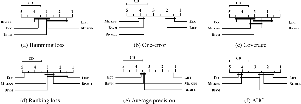
For each evaluation criterion, Friedman test at 0.05 significance level (five algorithms, sixteen data sets) rejects the null hypothesis of "equal" performance, which leads to the use of post-hoc tests to find out which algorithms actually differ. Specifically, Nemenyi test is utilized where the performance of two algorithms is significantly different if their average ranks over all data sets differ by at least one critical difference (CD). Figure 1 gives the CD diagrams [Demˇsar, 2006] for each evaluation criterion, where the average rank of each comparing algorithm is marked along the axis (lower ranks to the right). Groups of algorithms that are not significantly different according to Nemenyi test are connected with a thick line. The critical difference (CD=1.525 at 0.05 significance level) is also shown above the axis in each subfigure.
To summarize, out of all the 24 comparisons (4 algorithms to compare × 6 criteria), LIFT achieves statistically comparable performance in only 33% cases, i.e. the 8 comparisons against ML-KNN on hamming loss (Fig.1 a), against ECC on one-error (Fig.1 b), against BSVM and BP-MLL on coverage (Fig.1 c), on ranking loss (Fig.1 d), and on AUC (Fig.1 f). Rather impressively, LIFT achieves statistically superior performance in all the other 67% cases and no algorithms have once outperformed LIFT. These results clearly validate the superior effectiveness of our approach to the other wellestablished multi-label learning algorithms.
5 Conclusion
The major contributions of our work are two-fold: 1) A new strategy to multi-label learning via label-specific features is proposed, which suggests a new direction for learning from multi-label data; 2) A simple algorithm named LIFT is designed to justify the proposed strategy, whose effectiveness is thoroughly validated based on extensive comparative studies.
In the future, it is interesting to see whether LIFT can be further improved by incorporating label correlations into its label-specific features construction step as well as classification models induction step. Furthermore, designing other ways to fulfill the strategy of label-specific features is a direction very worth studying.
Acknowledgments
The author wishes to thank the anonymous reviewers for their helpful comments and suggestions.
@inproceedings{ijcai2011p270,
  title     = {LIFT: Multi-Label Learning with Label-Specific Features},
  author    = {Zhang, Min-Ling},
  booktitle = {Proceedings of the Twenty-Second International Joint Conference on
               Artificial Intelligence, {IJCAI-11}},
  publisher = {AAAI Press/International Joint Conferences on Artificial Intelligence},
  editor    = {Toby Walsh},
  pages     = {1609--1613},
  year      = {2011},
  month     = {7},
  doi       = {10.5591/978-1-57735-516-8/IJCAI11-270},
  url       = {https://doi.org/10.5591/978-1-57735-516-8/IJCAI11-270},
}
TY - CPAPER TI - LIFT: Multi-Label Learning with Label-Specific Features AU - Zhang, Min-Ling T2 - Proceedings of the Twenty-Second International Joint Conference on Artificial Intelligence, IJCAI-11 PB - AAAI Press/International Joint Conferences on Artificial Intelligence PY - 2011 SP - 1609 EP - 1613 DO - 10.5591/978-1-57735-516-8/IJCAI11-270 UR - https://doi.org/10.5591/978-1-57735-516-8/IJCAI11-270 ER -Copied
Machine-readable versions of this paper, for tools and AI agents:





