
Matrix Co-Factorization on Compressed Sensing
Proceedings of the Twenty-Second International Joint Conference on Artificial Intelligence. Pages 1595-1601.
https://doi.org/10.5591/978-1-57735-516-8/IJCAI11-268
© 2011 International Joint Conferences on Artificial Intelligence
Abstract
In this paper we address the problem of matrix factorization on compressively-sampled measurements which are obtained by random projections. While this approach improves the scalability of matrix factorization, its performance is not satisfactory. We present a matrix co-factorization method where compressed measurements and a small number of uncompressed measurements are jointly decomposed, sharing a factor matrix. We evaluate the performance of three matrix factorization methods in terms of Cram{'e}r-Rao bounds, including: (1) matrix factorization on uncompressed data (MF); (2) matrix factorization on compressed data (CS-MF); (3) matrix co-factorization on compressed and uncompressed data (CS-MCF). Numerical experiments demonstrate that CS-MCF improves the performance of CS-MF, emphasizing the useful behavior of exploiting side information (a small number of uncompressed measurements).
- [Candes and Tao, 2006] E. Candes and T. Tao. Near opti- mal signal recovery from random projections: Universal encoding strategies? IEEE Transactions on Information Theory, 52(12):5406-5425, 2006.
- [Donoho, 2006] D. L. Donoho. Compressed sensing. IEEE Transactions on Information Theory, 52(4):1289-1306, 2006.
- [Jolliffe, 2002] I. T. Jolliffe. Principal Component Analysis. Spinger-Verlag, 2 edition, 2002.
- [Kay, 1993] S. M. Kay. Fundamentals of Statistical Signal Processing: Estimation Theory. Prentice Hall, 1993.
- [Koren et al., 2009] Y. Koren, R. Bell, and C. Volinsky. Ma- trix factorization techniques for recommender systems. IEEE Computer, 42(8):30-37, 2009.
- [Lee and Choi, 2009] H. Lee and S. Choi. Group nonnega- tive matrix factorization for EEG classification. In Pro- ceedings of the International Conference on Artificial In- telligence and Statistics (AISTATS), Clearwater Beach, Florida, 2009.
- [Lee and Seung, 1999] D. D. Lee and H. S. Seung. Learning the parts of objects by non-negative matrix factorization. Nature, 401:788-791, 1999.
- [Lee et al., 2010] H. Lee, J. Yoo, and S. Choi. Semi- supervised nonnegative matrix factorization. IEEE Signal Processing Letters, 17(1):4-7, 2010.
- [O'Grady and Rickard, 2008] P. D. O'Grady and S. T. Rickard. Non-negative matrix factorisation of compress- ibely sampled non-negative signals. In Proceedings of the 8th IMA International Conference on Mathematics in Sig- nal Processing, Cirencester, UK, 2008.
- [Singh and Gordon, 2008] A. P. Singh and G. J. Gordon. Re- lational learning via collective matrix factorization. In Proceedings of the ACM SIGKDD Conference on Knowl- edge Discovery and Data Mining (KDD), Las Vegas, Nevada, 2008.
- [Smaragdis and Brown, 2003] P. Smaragdis and J. C. Brown. Non-negative matrix factorization for polyphonic music transcription. In Proceedings of IEEE Workshop on Appli- cations of Signal Processing to Audio and Acoustics, pages 177-180, New Paltz, NY, 2003.
- [Srebro et al., 2005] N. Srebro, J. D. M. Rennie, and T. Jaakkola. Maximum-margin matrix factorization. In Advances in Neural Information Processing Systems (NIPS), volume 17. MIT Press, 2005.
- [Xu et al., 2003] W. Xu, X. Liu, and Y. Gong. Docu- ment clustering based on non-negative matrix factoriza- tion. In Proceedings of the ACM SIGIR Conference on Research and Development in Information Retrieval (SI- GIR), Toronto, Canada, 2003.
- [Yoo and Choi, 2008] J. Yoo and S. Choi. Orthogonal non- negative matrix factorization: Multiplicative updates on Stiefel manifolds. In Proceedings of the 9th International Conference on Intelligent Data Engineering and Auto- mated Learning (IDEAL), Daejeon, Korea, 2008.
- [Yoo and Choi, 2009] J. Yoo and S. Choi. Weighted nonneg- ative matrix co-tri-factorization for collaborative predic- tion. In Proceedings of the 1st Asian Conference on Ma- chine Learning (ACML), Nanjing, China, 2009.
- [Yoo and Choi, 2010] J. Yoo and S. Choi. Orthogonal non- negative matrix-tri-factorization for co-clustering: Multi- plicative updates on stiefel manifolds. Information Pro- cessing and Management, 46(5):559-570, 2010.
- [Yoo et al., 2010] J. Yoo, M. Kim, K. Kang, and S. Choi. Nonnegative matrix partial co-factorization for drum source separation. In Proceedings of the IEEE Interna- tional Conference on Acoustics, Speech, and Signal Pro- cessing (ICASSP), Dallas, Texas, 2010.
- [Yu et al., 2005] K. Yu, S. Yu, and V. Tresp. Multi-label in- formed latent semantic indexing. In Proceedings of the ACM SIGIR Conference on Research and Development in Information Retrieval (SIGIR), Salvador, Brazil, 2005.
- [Zhu et al., 2007] S. Zhu, K. Yu, Y. Chi, and Y. Gong. Com- bining content and link for classification using matrix fac- torization. In Proceedings of the ACM SIGIR Conference on Research and Development in Information Retrieval (SIGIR), Amsterdam, The Netherlands, 2007.
References were extracted automatically from the PDF and may contain errors.
Full text extracted automatically from the PDF; figures, tables and equations may differ. The PDF is the version of record.
1 Introduction
Matrix factorization is a decomposition method where a data matrix X ∈ RM×N is approximated as a product of two or more factor matrices which uncover the latent structure of the data. The 2-factor decomposition seeks latent factor matrices U ∈ RM×K and V ∈ RN×K which minimize the following objective function
where ‖ · ‖F denotes the Frobenious norm. When columns in X are treated as data points in M-dimensional space, U and V are referred to be as basis matrix and encoding matrix, respectively. Exemplary matrix factorization methods include principal component analysis (PCA) [Jolliffe, 2002], nonnegative matrix factorization (NMF) [Lee and Seung, 1999], probabilistic matrix factorization (PMF) [Srebro et al., 2005], to name a few. Matrix factorization has established itself as a powerful technique in various applications such as collaborative prediction [Koren et al., 2009], document clustering [Xu et al., 2003; Yoo and Choi, 2010], music transcription [Smaragdis and Brown, 2003], and brain wave analysis [Lee and Choi, 2009]. In some of these applications such as collaborative prediction, the data matrix is sparse since most of entries are missing or unobserved. Thus, matrix factorization methods can be applied to a large scale problem without much extra care, since only observed elements are used for learning. On the other hand, data matrix is dense in some applications where spectrograms of music or brain wave data are analyzed. In such applications, it is not easy to handle large-scale data.
Compressed sensing is a new sensing/sampling paradigm which ensures near-optimal recovery of sparse signals from a small number of linear measurements [Donoho, 2006; Candes and Tao, 2006]. Compressed sensing is a promising approach to handling a large-scale dense data matrix since it is allowed to perform a processing (learning or data analysis) in the compressed domain (in which a compressivelysampled matrix is much smaller than the original input data matrix in size) rather than in the ambient space. Let Y ∈ RP×N be the compressively-sampled data matrix which is obtained by Y = ΦX, in which Φ ∈ RP×M is a linear sensing matrix which is often given by a random projection. A direct application of the compressed sensing framework to matrix factorization, referred to as CS-MF, yields the following objective function
CS-MF determines U and V which minimize (2), improving the scalability since Y and Φ requires less space in storage, compared to X. Recently, nonnegative matrix factorization (NMF) in the compressed domain, referred to as CS-NMF, was presented in [O'Grady and Rickard, 2008], where (2) is minimized with nonnegativity constraints imposed on factor matrices U and V as well as the data matrix X. In contrast to the standard compressed sensing framework where U is known in advance, CS-MF or CS-NMF estimates both U and V in the compressed-domain, which degrades the reconstruction performance.
Matrix co-factorization (MCF) is a technique that decompose two or more data matrices jointly, sharing some factor matrices in factorizations. In addition to the data matrix, side information matrices are also considered for the joint decomposition, including label information [Yu et al., 2005; Lee et al., 2010], link information [Zhu et al., 2007], intersubject variations [Lee and Choi, 2009], and spectrograms of music [Yoo et al., 2010]. MCF was also applied to the general entity-relationship models [Singh and Gordon, 2008; Yoo and Choi, 2009] to learn the characteristics of each entity from the relationships. In this paper we present a method of MCF on compressively-sampled data, referred to as CSMCF, where we decompose the compressed data matrix and a small portion of uncompressed original data jointly in order to improve the performance of matrix factorization in the compressed domain. We compute the Cram´er-Rao bound (CRB) for matrix factorization on uncompressed data (MF), CS-MF, and CS-MCF in the case of Gaussian likelihood, showing that CS-MCF indeed improves the performance over CS-MF in terms of the reconstruction quality. We consider alternating least squares (ALS) algorithms for MF, CS-MF, and CS-MCF. In addition, we also consider multiplicative updates, as in NMF, comparing NMF, CS-NMF (NMF in the compressed domain), and CS-NMCF (nonnegative matrix cofactorization in the compressed domain with small uncompressed information).
2 Matrix Co-Factorization on Compressively Sampled Data
Compressed sensing [Donoho, 2006; Candes and Tao, 2006] is a new framework which performs the measurement and compression simultaneously to reduce computation required in the measurement process. The fundamental theoretical results of compressed sensing is based on the sparsity of the representation of given data, which makes possible to reduce the required number of measurement less than the amount computed from the classical Shannon-Nyquist sampling theorem. Compressed sensing assumes that the basis which sparsely represents the given data is known, however, the appropriate representation basis for given data is usually not known in advance. In that cases we have to learn a representation matrix from a given data, however, the problem of learning representation basis from the compressed measurement has not been studied much.
Matrix factorization in the compressed domain considers a decomposition of the compressively-sampled data matrix Y = ΦX where Φ ∈ RP×M is a random projection. Thus given X and Φ, CS-MF seeks Y ≈ ΦUV ⊤, determining factor matrices U and V which minimizes (2). In contrast to the compressed sensing framework where the basis matrix U is known in advance, CS-MF should estimate both U and V given compressed data Y . We believe that this explains the poor reconstruction performance of CS-MF in our experiments.
Now we explain matrix co-factorization in the compressed domain with exploiting partial uncompressed data. We partition the data matrix X ∈ RM×N into two sub-matrices Xc ∈ RM×C and Xu ∈ RM×(N-C) . Assuming that C > (N-C), the sub-matrixXc is compressed by a random projection Φ, leading to Y = ΦXc with the abuse of notation. CS-MCF considers a joint decomposition of the compressed data matrix Y and partial uncompressed data Xu, minimizing the following objective function:
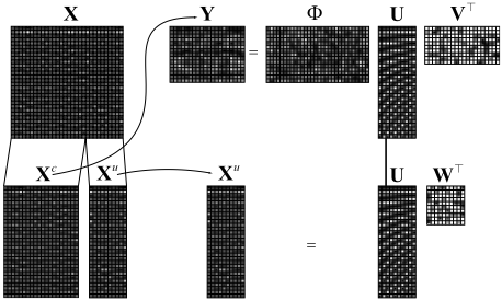
where the factor matrix U ∈ RM×K is shared, capturing the common characteristics in representing both Y and Xu, and V ∈ RC×K and W ∈ R(N-C)×K capture individual characteristics. The parameter λ controls the balance between two decomposition. Pictorial illustration of CS-MCF is given in Fig. 1.
2.1 ALS Updates
ALS updates for U, V ,W are easily derived by solving
for U, V ,W, respectively, and the corresponding gradients of (3) are calculated as
leading to ALS updates
where IM is the identity matrix with size M ×M, vec(U) = [u⊤1 , . . . , u⊤K ]⊤ is the 'vec' operator which creates a column vector from the matrix U by stacking columns of U, and ⊗ denotes the Kronecker product (tensor product).
| Model | Updates | Model | Updates |
|---|---|---|---|
| MF | U ← XV (V ⊤V )-1 V ←X⊤U(U ⊤U)-1 | NMF | U ←U ⊙ XV UV ⊤V V ←V ⊙ X⊤U V U ⊤U |
| CS-MF | vec(U) ← ((V ⊤V ) ⊗ (Φ⊤Φ))-1 vec(Φ⊤Y V ) V ← Y ⊤ΦU(U ⊤Φ⊤ΦU)-1 | CS-NMF | U ←U ⊙ Φ⊤Y V Φ⊤ΦUV ⊤V V ←V ⊙ Y ⊤ΦU V U ⊤Φ⊤ΦU |
| CS-MCF | vec(U) ← ((V ⊤V ) ⊗ (Φ⊤Φ) + λ(W ⊤W) ⊗IM)-1 vec(Φ⊤Y V + λXuW ) V ← Y ⊤ΦU(U ⊤Φ⊤ΦU)-1 W ← Xu⊤U(U ⊤U)-1 | CS-NMCF | U ←U ⊙ Φ⊤Y V +λXu⊤W Φ⊤ΦUV ⊤V +λUW ⊤W V ←V ⊙ Y ⊤ΦU V U ⊤Φ⊤ΦU W ←W ⊙ Xu⊤U WU ⊤U |
2.2 Multiplicative Updates
As in NMF, we derive multiplicative updates for U, V ,W which iteratively minimize (3) with nonnegativity constraints imposed on factor matrices, given the nonnegative data matrix. Our derivation follows the technique used in [Yoo and Choi, 2008] where the gradient of an objective function J is decomposed as
where [ ∂L ∂Θ ]+ > 0 and [ ∂L ∂Θ ]- > 0, and then multiplicative updates for parameters Θ are given by
where ⊙ denotes Hadamard product (element-wise product) and the division is done in an element-wise manner. Applying this technique to the minimization of (3) yields
ALS or multiplicative updating algorithms for MF and CSMF are also derived in the same way, which are summarized in Table 1.
3 Cram´er-Rao Bounds
We calculate the Cram´er-Rao bound (CRB) to evaluate the performance of matrix factorization, CS-MF, and CS-MCF. CRB [Kay, 1993] provide the lower bound of the variance of unbiased estimators of a deterministic parameter in the following form,
where θ is the estimated parameter of the model, ˜θ is the true value of the parameter, A ≥ B denotes that A-B is the positive semi-definite matrix, and I is the Fisher information matrix, each element of which is computed by
where p(x|θ) is the likelihood. In the case of matrix factorization, we have factor matrices U ∈ RM×K and V ∈ RN×K as the parameters for the model, so θ becomes
where ui and vj represent the column vector consist of the elements in the i-th and j-th row of U and V , respectively. Then, the Fisher information matrix has the following representation,
where each part is computed for the corresponding parameter, for example,
where [A]i,j represents the (i, j )-th element in the matrix A. The Fisher information matrix of CS-MCF has a different parametrization with the matrix U, V and W, which is
| MF | CS-MF U V | CS-MCF U V W | |
|---|---|---|---|
| Graphical Model | X U V | Y X | Y u X c X |
| Likelihood | p(X|U, V ) = ∏j N(xj|Uvj,Σ) | p(Y |U, V ) = ∏j N(yj|ΦUvj,Σ) | p(Y , Xu |U, V ,W) = ∏j N (yj |ΦUvj , Σb) ∏k N (xuk |Uwk , Σa) |
| FIM IU IV IUV IW IUW IV W | (V ⊤Σ-1V ) ⊗IM (U ⊤Σ-1U) ⊗IN vec(UΣ-1 )vec(V )⊤ | (V ⊤V ) ⊗ (Φ⊤Σ-1Φ) (U ⊤Φ⊤Σ-1ΦU) ⊗IN vec(UΦ⊤Σ-1Φ)vec(V )⊤ | (V ⊤V ) ⊗ (Φ⊤Σ-1 a Φ) + (W ⊤Σ-1 b W) ⊗IM (U ⊤Φ⊤Σ-1 a ΦU) ⊗IC vec(U ⊤Φ⊤Σ-1 a Φ)vec(V )⊤ (U ⊤Σ-1 b U) ⊗IN-C vec(UΣ-1 b )vec(W)⊤ 0 |
| CRB (U known) | [IV ]-1 | [IV ]-1 | [ IV IVW I ⊤ VW IW ]-1 |
| CRB (U unknown) | [ IU IUV I ⊤ UV IV ]-1 | [ IU IUV I ⊤ UV IV ]-1 | ⎡⎣ IU IUV IUW I ⊤ UV IV IVW I ⊤ UW I ⊤ VW IW ⎤⎦-1 |
and each element of the parts is computed in the similar way to (6) and (7).
The CRB for matrix factorization, CS-MF and CS-MCF are computed in the following subsections. We use the maximum likelihood estimator (MLE), which is known to be asymptotically unbiased and efficient under mild regularity conditions [Kay, 1993]. The analysis is based on these asymptotic properties, assuming that there are sufficient number of samples. The models, computed Fisher information matrices and the form of CRB are summarized in Table 2.
Since the solution of the matrix factorization is not uniquely determined, the direct comparison between the estimated parameters and the ground-truth values is meaningless. Instead of directly comparing the parameters themselves, we use the expected reconstruction error
where ˜ Xij, ˜ui, and ˜ vj are the ground-truth values of the parameters, and Xij is the element of the reconstructed input matrix from the estimated parameters ui and vj. Although the factor matrices is not uniquely determined, the reconstruction error Eij is the same for all the possible decompositions. The lower bound for the reconstruction error is represented by using the variances of the estimators, such as
If we assume that the estimator is unbiased, the last term of the above equation becomes zero, and the remaining terms are lower-bounded by the computed CRB,
where [I -1 ]ui represents the part of the inverse Fisher information matrix corresponding to the position of Iui . Then, the error bound becomes
Note that if we assume that the basis matrix U is known in advance, we only have to deal with the parameter V . With the computation similar to the above, the lower bound of the reconstruction error is computed in the following form,
which is smaller than the case when the basis is unknown in the amount of the terms corresponding to U, which is ˜ v⊤j [I -1 ]ui ˜ vj +Tr {[I -1 ]ui [I -1 ]vj }.
3.1 Cram´er-Rao Bounds for Matrix Factorization
The Fisher information matrix is computed from the likelihood of the model. If we assume that the noise is additive and distributed as the Gaussian distribution, the model is written by
where Nij ∼ N(0, σ2 ), and N(μ, σ2 ) is the Gaussian distribution with mean μ and variance σ2 . Then, the likelihood of the model becomes
Calculation of IV
The derivative of the log-likelihoodwith respect to vj is computed by
where Σ = σ2 IM. If we differentiate above again with respect to vj′ , where j ′ ̸= j, the result becomes zero. If j ′ = j, then,
Therefore, the part of Fisher informationmatrix for V is computed by
Calculation of IU
In this case, we use the likelihood of the model having the following form,
where xi represents the i-th row of the input matrix X. The first derivative with respect to ui is computed as
Again, the second derivative becomes zero if i′ ̸= i, and if i′ = i,
Therefore, Fisher information matrix for U is written by
Calculation of IUV
To compute IUV , we differentiate (11) with respect to vj, which becomes
Since E{xijIK} = u⊤i vjIK, the first two terms of the above equation vanishes when we take the expectation. Therefore, the Fisher information matrix for U and V is written by
3.2 Cram´er-Rao Bound for CS-MF
We model the CS-MF with the following two-step procedure,
where [Na]i,j ∼ N(0, σ2 a) is the representation error and [Nb]i,j ∼ N(0, σ2 b ) is the measurement error. The likelihood is written by
where Σ = σ2 aΦΦ⊤ + σ2 b IP , where Φ ∈ RP×M .
Calculation of IV
The derivative of the log-likelihoodwith respect to vj is computed by
Differentiate again with vj′ becomes zero when j ′ ̸= j, and if j ′ = j, then
Therefore, the Fisher information matrix for V is computed by
Calculation of IU
The derivative with respect to ui is written by
The derivative of above equation with respect to ui′ is simplified by
which leads the Fisher information matrix for U to be
Calculation of IUV
If we differentiate (12) with respect to vj , we obtain
The first two terms disappear when we take the expectation, so the Fisher information matrix for U and V becomes
The theoretical bound of CS-MF is larger than that of matrix factorization. The main difference of the computed Fisher information matrix is from the change of the term Σ-1 of matrix factorization to the term Φ⊤Σ-1Φ. Note that the Σ-1 in the matrix factorization is
However, Φ⊤Σ-1Φ in the CS-MF is written by
This is usually smaller than the corresponding term in the matrix factorization. For example, if we assume that σ2 b = 0 and each element of sensing matrix is drawn independently from N (0, 1), we approximate the term using Φ⊤Φ ≈ PIM and ΦΦ⊤ ≈ MIP , such that
which is P/M times smaller than that part of matrix factorization (12). Since the CRB is calculated as the inverse of the Fisher information matrix, CS-MF has larger CRB than that of the matrix factorization.
3.3 Cram´er-Rao Bound for CS-MCF
The relations in CS-MCF are modeled as in the previous section, such that
where [Na]i,j ∼ N(0, σ2 a), [Nc]i,j ∼ N(0, σ2 a) and [Nb]i,j ∼ N(0, σ2 b ). In this case we have three parameters U, V , andW, so the Fisher information matrix is computed as
The likelihood is
where Σb = σ2 aΦΦ⊤ + σ2 b IP and Σa = σ2 aIM .
Calculation of IU
Differentiating the log-likelihood with respect to ui leads
Differentiating again with respect to ui′ yields
where i′ = i, and yields
where i′ ̸= i. Therefore, the Fisher information matrix for U becomes
Calculation of IV , IW, IUV , and IVW
IV , IW, IUV , and IVW are computed in the similar way as in matrix factorization and CS-MF, in the following forms,
Calculation of IV W
Fisher information matrix for V andW, IV W , becomes zero matrix of dimension CK × (N -C)K because the termW banishes in the derivative with respect to vj .
The Fisher information matrix of CS-MCF is the combination of the Fisher information matrix of matrix factorization and Fisher information matrix of CS-MF. The parameter V in matrix factorization and CS-MF is divided into V and W in CS-MCF. The IV and IUV in CS-MCF follows the form of the corresponding parts of CS-MF, but the IW and IUW follows the form of the corresponding parts of matrix factorization. Moreover, IU is the direct combination of the IU of matrix factorization and IU of CS-MF. In the previous section, we showed that in general the CRB of matrix factorization is smaller than the CRB of CS-MF, so this kind of combination leads smaller CRB than that of CS-MF.
4 Numerical Experiments
For the numerical experiments, we computed the bounds of the reconstruction performances using the equation (9), and compared them with the actual reconstruction performances of the algorithms listed in the Table 1. We also computed the bounds for the cases where we assume that the parameter U is known in advance (10). In that cases, the actual reconstruction performances were measured based on the modified algorithms, where the parameter U is fixed with the groundtruth values.
To compute the CRB, we have to know the ground-truth value of the parameters U, V , and W, which makes it difficult to use the real-world data where the ground-truth factor matrices are unknown. Therefore, we used synthetic data for the experiments. The factor matrices U ∈ ℜ100×10 , V ∈ ℜ100×10 and the sensing matrix Φ ∈ ℜ20×100 are randomly generated, and the input matrices were drawn from them with additive Gaussian noise. For the ALS-based algorithms, each element of the factor matrices and the sensing matrix is sampled from the Gaussian distribution with mean
0 and variance 1. For the multiplicative update algorithms which have the nonnegativity constraints, each element is sampled from a uniform distribution between 0 and 1. For the co-factorizations, 20 out of 100 columns were chosen for the uncompressed prior.
As a measure of the reconstruction performances, we used signal-to-noise ratio (SNR)
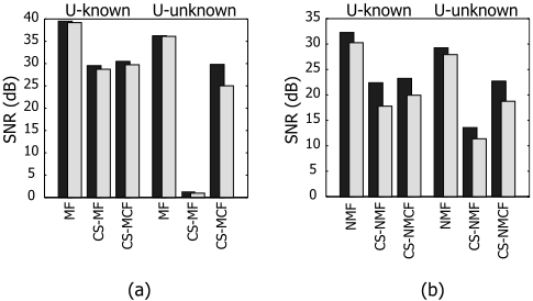
where ˜ X is the true value of the input matrix, U and V are the factor matrices obtained by running the algorithms. The SNRs were averaged over the 100 different trials (Figure 2). The bounds were better for the cases where the matrix U is known in advance, than the cases where the matrix U is unknown. This indicates that the estimation of both U and V is more difficult than the estimation of V only. The bounds of CS-MF and CS-NMF were seriously degraded compared to the bounds of MF and NMF, as well as the actual performances, especially for the cases that the matrix U is unknown. However, the co-factorization based methods showed much improved bounds, as well as the performances, compared to CS-MF and CS-NMF. The use of uncompressed prior as the side information actually helps to improve the reconstruction performance in the learning from the compressed data.
As an illustrative example, we ran the algorithms for the compressively sampled data on the cameraman image (Figure 3). We divided the image using 8-by-8 patches to build an input matrix, and compress each column into the size of 49. 25 % of the data is randomly selected to be used for the uncompressed prior. CS-MCF brought much better reconstruction result than the CS-MF.
5 Conclusions
We have presented a method for matrix co-factorization in the compressed domain where compressively-sampled data and partial uncompressed data were jointly decomposed, sharing a factor matrix. We calculated CRBs for three matrix factorization methods (MF, CS-MF, CS-MCF) in the case of Gaussian likelihood, showing that CS-MCF improves the reconstruction performance over CS-MF. Numerical experiments on image confirmed the better performance of CS-MCF over CS-MF.
Acknowledgments: This work was supported by NIPAMSRA Creative IT/SW Research Project, the Converging Research Center Program funded by Korea MEST (No. 2010K001171), NIPA ITRC Support Program (NIPA-2011C1090-1131-0009), and NRF WCU Program (R31-2010000-10100-0).
@inproceedings{ijcai2011p268,
  title     = {Matrix Co-Factorization on Compressed Sensing},
  author    = {Yoo, Jiho and Choi, Seungjin},
  booktitle = {Proceedings of the Twenty-Second International Joint Conference on
               Artificial Intelligence, {IJCAI-11}},
  publisher = {AAAI Press/International Joint Conferences on Artificial Intelligence},
  editor    = {Toby Walsh},
  pages     = {1595--1601},
  year      = {2011},
  month     = {7},
  doi       = {10.5591/978-1-57735-516-8/IJCAI11-268},
  url       = {https://doi.org/10.5591/978-1-57735-516-8/IJCAI11-268},
}
TY - CPAPER TI - Matrix Co-Factorization on Compressed Sensing AU - Yoo, Jiho AU - Choi, Seungjin T2 - Proceedings of the Twenty-Second International Joint Conference on Artificial Intelligence, IJCAI-11 PB - AAAI Press/International Joint Conferences on Artificial Intelligence PY - 2011 SP - 1595 EP - 1601 DO - 10.5591/978-1-57735-516-8/IJCAI11-268 UR - https://doi.org/10.5591/978-1-57735-516-8/IJCAI11-268 ER -Copied
Machine-readable versions of this paper, for tools and AI agents:





