
Dealing with Concept Drift and Class Imbalance in Multi-Label Stream Classification
Proceedings of the Twenty-Second International Joint Conference on Artificial Intelligence. Pages 1583-1587.
https://doi.org/10.5591/978-1-57735-516-8/IJCAI11-266
© 2011 International Joint Conferences on Artificial Intelligence
Abstract
Data streams containing objects that are (or can be) associated with more than one label at the same time are ubiquitous. In spite of its important applications, classification of streaming multi-label data is largely unexplored. Existing approaches try to tackle the problem by transferring traditional single-label stream classification practices to the multi-label domain. Nevertheless, they fail to consider some of the unique properties of the problem such as within and between class imbalance and multiple concept drift. To deal with these challenges, this paper proposes a novel multi-label stream classification approach that employs two windows for each label, one for positive and one for negative examples. Instance-sharing is exploited for space efficiency, while a time-efficient instantiation based on the k-Nearest Neighbor algorithm is also proposed. Finally, a batch-incremental thresholding technique is proposed to further deal with the class imbalance problem. Results of an empirical comparison against two other methods on three real world datasets are in favor of the proposed approach.
- [Domingos and Hulten, 2000] P. Domingos and G. Hulten. Mining high-speed data streams. In Proceedings of the 6th ACM SIGKDD International Conference on Knowl- edge Discovery and Data Mining, pages 71-80, 2000.
- [Gaber et al., 2007] M. Gaber, A. Zaslavsky, and S. Krish- naswamy. A survey of classification methods in data streams. In Data Streams: Models and Algorithms, chap- ter 3, pages 39-59. Springer, 2007.
- [Gama et al., 2009] J. Gama, R. Sebastião, and P.P. Ro- drigues. Issues in evaluation of stream learning algorithms. In Proceedings of the 15th ACM SIGKDD International Conference on Knowledge Discovery and Data Mining, pages 329-338, 2009.
- [Gao et al., 2007] J. Gao, W. Fan, J. Han, and P.S. Yu. A general framework for mining concept-drifting data streams with skewed distributions. In Proceedings of the 7th SIAM International Conference on Data Mining (SDM'07), pages 3-14, 2007.
- [Godbole and Sarawagi, 2004] S. Godbole and S. Sarawagi. Discriminative methods for multi-labeled classification. In Proceedings of the 8th Pacific-Asia Conference on Knowl- edge Discovery and Data Mining, pages 22-30, 2004.
- [Klinkenberg and Joachims, 2000] R. Klinkenberg and T. Joachims. Detecting concept drift with support vector machines. In Proceedings of the 17th International Conference on Machine Learning, pages 487-494, 2000.
- [Lewis et al., 2004] D.D. Lewis, Y. Yang, T.G. Rose, and F. Li. Rcv1: A new benchmark collection for text catego- rization research. Journal of Machine Learning Research, 5:361-397, December 2004.
- [Qu et al., 2009] W. Qu, Y. Zhang, J. Zhu, and Q. Qiu. Min- ing Multi-label Concept-Drifting Data Streams Using Dy- namic Classifier Ensemble. In Proceedings of the 1st Asian Conference on Machine Learning, pages 308-321, 2009.
- [Read et al., 2009] J. Read, B. Pfahringer, G. Holmes, and E. Frank. Classifier chains for multi-label classification. In Proceedings of ECML PKDD '09, pages 254-269, 2009.
- [Read et al., 2010] J. Read, A. Bifet, G. Holmes, and B. Pfahringer. Efficient multi-label classification for evolv- ing data streams. Technical Report, April 2010.
- [Srivastava and Zane-Ulman, 2005] A.N. Srivastava and B. Zane-Ulman. Discovering recurring anomalies in text reports regarding complex space systems. In Proceedings of IEEE Aerospace Conference, pages 3853 -3862, 2005.
- [Tsoumakas et al., 2010] G. Tsoumakas, I. Katakis, and I. Vlahavas. Mining multi-label data. In Data Mining and Knowledge Discovery Handbook, chapter 34, pages 667- 685. Springer, 2nd edition, 2010.
- [Ueno et al., 2006] K. Ueno, X. Xi, E. Keogh, and D.-J. Lee. Anytime classification using the nearest neighbor algo- rithm with applications to stream mining. IEEE Interna- tional Conference on Data Mining, pages 623-632, 2006.
- [Wenerstrom and Giraud-Carrier, 2006] B. Wenerstrom and C. Giraud-Carrier. Temporal data mining in dynamic fea- ture spaces. In Proceedings of the Sixth International Con- ference on Data Mining, ICDM '06, pages 1141-1145, Washington, DC, USA, 2006. IEEE Computer Society.
References were extracted automatically from the PDF and may contain errors.
Full text extracted automatically from the PDF; figures, tables and equations may differ. The PDF is the version of record.
1 Introduction
Multi-label stream classification (MLSC) has emerged recently as an extension to conventional stream classification in response to applications where arriving data instances can or must acquire more than one label. This typically happens either because the labels are orthogonal or because it is not practical to define labels that are completely distinct and intuitive at the same time. Orthogonal labels are encountered e.g. in the categorization of incoming mails or enterprize documents: such instances may be relevant to a thematic label, as well as to a label concerning confidentiality. Such classes are a priori orthogonal, but correlations may be encountered (e.g. instances belonging to some theme are confidential). Overlapping classes are typical in news. For example, an article about the Fukushima nuclear plant could be annotated with labels like "nuclear crisis", "Asia-Pacific news", "energy" and "environment".
Multi-label classification of static data enjoys increased attention in recent years. An overview of the domain, including discussion of applications can be found in [Tsoumakas et al., 2010]. Solutions for static data do not readily transfer to stream scenarios though, since they assume static concepts and availability of all data for learning. On the other hand, research on single-label stream classification has contributed several powerful algorithms (cf. [Gaber et al., 2007] for an overview) that exhibit good predictive power and fast adaptation to concept drift. In principle, drift adaptation encompasses monitoring the distribution of positive and negative examples within some window, and discarding old examples when the most recent data indicate a change in the distribution. Some of these solutions have been extended to the multi-label case (e.g. [Qu et al., 2009]), without however explicitly addressing a number of challenges that are specific to multi-label streams.
A multi-label data stream contains separate multiple targets (concepts), and it is impractical to assume that all of themwill start drifting simultaneously or at the same rate. Essentially, each concept is likely to exhibit its own drift pattern. Another challenge of multi-label data is the class imbalance problem: each label has usually more negative than positive examples, but still some labels have much more positive examples than others. If a single window is used, it is expected that some labels will have enough examples for learning the positive class, but many labels may have little or even no positive examples.
We present a new approach that deals with the above challenges of MLSC. Our new Multiple Windows (MW) method maintains two fixed-size windows per label, one for positive and one for negative examples. This is accomplished in a space-efficient way through instance-sharing between windows. In addition, we present a time-efficient instantiation of this method, using k-Nearest-Neighbors (kNN) as the base classifier for each label. Class imbalance is further tackled using a new batch-incremental thresholding technique that accurately translates the probabilistic estimates for each label to bipartitions.
The rest of the paper is organized as follows. In section 2, we discuss existing work on multi-label stream classification and further relevant literature. Section 3 presents our contributions. It is followed by the empirical evaluation in section 4. The last section concludes our study.
2 RelatedWork
One of the first methods for MLSC is [Qu et al., 2009]. It assumes that stream instances arrive in chunks of size S and builds an ensemble of K classifiers, on K successive chunks. To deal with concept drift, every S examples the oldest model is replaced by a model built on the latest chunk. The authors used stacked binary relevance [Godbole and Sarawagi, 2004] to learn from each chunk, but the method could be coupled with any batch multi-label learner.
Another work dealing with multi-label streams is [Read et al., 2010]. It presents a framework for generating synthetic multi-label data streams along with a novel MLSC method based on the Hoeffding Tree [Domingos and Hulten, 2000], a popular decision tree classifier for single-label streams. Their method extends the Hoeffding Tree by using a multi-label definition of entropy and by training multi-label classifiers at the leaves of the tree. However, it does not offer drift adaptation, hence is not suitable for classifying evolving multi-label streams.
The aforementioned approaches try to tackle MLSC by combining existing stream and multi-label classification methods but they do not deal explicitly with the special characteristics of a multi-label stream such as independent concept drift for each label (or group of labels) and skewness in the distribution of positive and negative examples for most of the labels.
In single-label data streams, most approaches assume balanced distributions of positive and negative examples. One of the exceptions is the method of [Gao et al., 2007]. This method processes the stream instances in batches. It tries to build balanced training sets as follows: all positive examples are kept, while the negative examples of the latest chunk are undersampled, and organized (together with the positive ones) into multiple disjoint samples. Then, an ensemble of classifiers is trained, which is completely rebuilt upon the arrival of the latest chunk. Ensemble re-learning is computationally expensive, though. Moreover, retaining all positive examples may 1) prevent the learner from adapting properly to drift and 2) prohibitively increase re-training time.
We follow a similar strategy to deal with label skewness in multi-label streams but we impose a limit in the number of positive examples that we keep for each label. This way we overcome the aforementioned disadvantages of the method of [Gao et al., 2007] and make it more suitable for multi-label streams where each label has each own degree of skewness. Furthermore, our method is instance-incremental and thus allows faster adaptation to drift and avoids the computational overhead of rebuilding the model from scratch.
3 Our Contributions
3.1 AMultipleWindows Approach
Our approach starts from a mainstream idea for learning from single-label concept-drifting data streams, that of the movingwindow [Klinkenberg and Joachims, 2000]. As its name implies, this idea is about maintaining a classifier that is trained from a moving window of recent examples.
A couple of issues can arise if we attempt to apply this idea to multi-label data: a) Each label constitutes a different learning problem, including a different rate of concept drift. b) The distribution of positive and negative examples for most labels will be skewed, and the negative examples are expected to dominate, so that the few positive examples will be insufficient for learning the positive class for some of the labels. An option here is to increase the size of the window, allowing a sufficient number of positive examples for all labels. However, this would increase the probability of concept drift occurrence in the window.
To deal with the above issues we propose the following approach. We associate each label with two fixed size instancewindows, one for positive and one for negative examples. A new training example is placed in the positive (negative) windows of its relevant (irrelevant) labels. The size np of the positive windows is a parameter of the approach and should be (1) large enough to allow learning an accurate model (2) small enough to reduce the probability of concept drift in the window. The number of examples in the negative windows, nn, is determined using the formula nn = ⌈np/r⌉ where r is another parameter of the approach, called distribution ratio, with the role of balancing the distribution of positive and negative examples in the union of the two windows and typical values between 0.3 and 0.7 [Gao et al., 2007].
Compared to a window-based approach that would use a single window for a label, our approach effectively oversamples the positive and undersamples the negative examples for all labels whose ratio of positive to negative examples in the single window is less than the desirable ratio r. The oversampling is achieved by adding the most recent positive examples that appear prior to that window and the undersampling by retaining only the most recent negative examples. Figure 1 contrasts the two approaches.
Our technique reduces the high variance caused by the insufficient positive examples available to a classifier operating in a single window, leading to reduced classification error. In the case of concept drift, the bias may increase by the introduction of old positive examples caused by oversampling. However, this increase is expected to be small because the negative examples are expected to always be current.
We follow the binary relevance (BR) approach, since we transform the multi-label problem into multiple binary problems and tackle each problem independently. BR has been criticized in the past for ignoring potential underlying label correlations, but, in the meanwhile, there are BR-based methods that overcome this limitation (e.g. [Read et al., 2009]). We use the independent modeling of BR, because it allows us to effectively handle the expected differences in frequency and concept drift between the labels. BR offers also a number of further advantages: a) it can be combined with any binary classification algorithm, b) it can easily handle the appearance of new labels by training a new corresponding binary classifier, c) it can be easily parallelized to achieve a constant time complexity with respect to the number of labels.
| Stream | n | p | n | n | p | p | n | n | n | n | n | n | n | p | n | n | p | n | n n |
|---|---|---|---|---|---|---|---|---|---|---|---|---|---|---|---|---|---|---|---|
| Typical window-based method | * | * | * | * * | * | * | * | * | * | ||||||||||
| Our approach | * | * | * | * * | * | * | * | * | * |
Space-Efficient Implementation of Multiple Windows
In the following, we describe a space-efficient implementation of the proposed multiple windows scheme. In particular, we discuss the update of the windows when a new example arrives. The pseudocode of the update method is listed in Algorithm 1. Table 1 summarizes the notation used in the pseudocode.
| Notation | Description |
|---|---|
| xi Yi = {l1, .., l|Yi|} L = {l1, ..., l|L|} B = {(x1, Y1), .., (xn, Yn)} Qp = {Qpl1 , .., Qp|L| } Qn = {Qnl1 , .., Qn|L| } np r k | The ith stream instance The label set of xi The set of observed labels Shared buffer of examples Positive windows Negative windows Size of positive windows Distribution ratio # of nearest neighbors |
Algorithm 1 is invoked for each arriving labeled instance, in order to update the positive and negative windows of each label. Each window is implemented as a queue. When the UpdateWindow function is called (lines 4, 6, 10), we insert the current instance in the queue and push the oldest instance out of the queue if it is full. The positive and negative queues store only references to the original instances, which are stored only once in the shared buffer B. Every time an instance is removed from a queue, the algorithm updates a counter which holds the number of queues in which the instance is still present. If the counter becomes 0, the instance is also deleted from the shared buffer. Notice that when a labeled instance contains a label which appears for the first time, then the set of observed labels L is updated and a new positive and a new negative queue are created for this label (lines 8-9). Thus the algorithm automatically handles unseen labels.
The size of the shared buffer |B| determines the spacecomplexity of the method and depends on the following factors: (1) the size of the positive windows, (2) the number of observed labels and (3) the overlap between the labels. The value np ∗ |L| is the theoretical maximum for |B| and is reached if there is no overlap among the labels. The positive window of a label with no co-occurrences with other labels shares 0 examples with the other windows. On the other hand, np∗|L| C , where C is the average number of labels per instance, is a lower bound for |B|. It represents the case where the average C is evenly distributed among the labels. In practise the overlap is never evenly distributed (there are groups
Algorithm 1: UpdateModel (xi,Yi) Input: B, Qp , Qn , L Output: The updated model 1 B ←B ∪ {(xi, Yi)} 2 foreach lj ∈ L∪ Yi do 3 if lj ∈ L∩ Yi then 4 Qplj ← UpdateWindow(xi ,Qplj ) 5 else if lj ∈ L \ Yi then 6 Qnlj ← UpdateWindow(xi ,Qnlj ) 7 else 8 L ← L ∪ {lj }, Qplj ← null, Qnlj ← null 9 Qp ←Qp ∪Qplj , Qn ←Qn ∪Qnlj 10 Qplj ← UpdateWindow(xi ,Qplj )of labels with higher overlap than others) and |B| grows when the distribution of co-occurrences is skewed. The size of the negative windows nn does not affect |B| since we can find negative examples to fill all the negative windows in the latest nn/(1-maxfr) stream instances, where maxfr is the frequency of the most frequent label. Our experiments (not reported here due to space limitations) verify that |B| lies between the above bounds.
3.2 An Efficient kNN-based Implementation
We chose kNN to instantiate the proposed multiple windows approach for the following reasons:
- kNN is an incremental classifier. As such it can incorporate new instances in the model and discard old ones without needing to be rebuilt from scratch. The method could also be coupled with non-incremental base classifiers, but this would require rebuilding the classification model in regular time periods. This would reduce the ability of the method to adapt quickly to sudden concept changes, as it would require to wait for a batch of instances to arrive before updating the model.
- kNN is a method which makes no assumptions on the form of the data distribution and learns the structure of the hypothesis directly from the training data. In stream classification, we usually have no prior knowledge about the data distribution and additionally the distribution may evolve over time.
- kNN is a fast algorithm with proven success in singlelabel data streams [Ueno et al., 2006].
We further developed an efficient kNN implementation of the prediction method that makes a single pass over the examples of the shared buffer to calculate the distance between the unlabeled instance and any of the examples in the shared buffer only once. As shown in Algorithm 2, instead of performing nearest neighbor search in the instances of Qplj ∪ Qnlj for every label lj , we calculate the distances of all instances in B to the test instance only once and sort B on these distances (line 5). Then we scan the sorted list from top to bottom and gather the votes for each label until all the nearest neighbors have been found.
Algorithm 2: MakePrediction(xi) Input: B,Qp , Qn , L, k Output: confidence[lj]: a confidence score for each label 1 // initialize counters 2 totalNNCounter = |L| ∗ k 3 foreach lj ∈ L do 4 NNCounter[lj] = k 5 BSort = sort(B,xi) // Sort instances in B by distance from xi 6 for m← 1 to |Bsort| do 7 if totalNNCounter == 0 then 8 break 9 foreach lj ∈ L do 10 if NNCounter[lj] == 0 then 11 continue 12 if BSort[m] ∈ Qplj ∪Qnlj then 13 NNCounter[lj] = NNCounter[lj] - 1 14 totalNNCounter = totalNNCounter - 1 15 if lj ∈ Qplj then 16 votes[lj ]++ 17 foreach lj ∈ L do 18 confidence[lj] = votes[lj] /k3.3 A Batch-Incremental ThresholdingMethod
Each kNN classifier actually computes an estimation of the probability of the corresponding label being relevant, which is transformed into a hard 0/1 classification via an implicit 0.5 threshold. This is true for other classifiers as well, like logistic regression (which is not incremental) and naive Bayes (which is incremental).
However, when data are characterized by class imbalance, the typical 0.5 threshold is often an improper choice. We therefore, propose a novel batch-incremental thresholding method which computes a different threshold for each label independently of a specific evaluation measure.
The method is simple: we calculate the frequency of each label and store the confidence scores given for each label every n instances. We then sort the confidence scores and select as a threshold for each label the value which would more accurately approximate the observed label frequency in these n instances. We use these threshold values for the next n instances and re-calculate the thresholds.
The only report of another incremental thresholding method for multi-label classifiers is found in [Read et al., 2010] where they incrementally adjust a common threshold for all labels so that the predicted label cardinality matches the actual one. We rather use a threshold for each label, in order to reduce the impact of class imbalance which is known to negatively affect the performance of BR-based classifiers.
4 Empirical Results
4.1 Datasets
We experimented on three large real-world textual multi-label datasets. Table 2 presents the main statistical properties of these datasets.
The tmc2007 dataset [Srivastava and Zane-Ulman, 2005] comes from a competition organized by the text mining workshop of the 7th SIAM international conference on data mining. The original data comprised 28596 aviation safety reports in free text form, annotated with one or more out of 22 problem types that appear during flights. The imdb dataset contains 120919 movie plot text summaries from the Internet Movie Database, labeled with one or more out of 28 genres [Read et al., 2009]. The reuters (rcv1v2) data set is a well known benchmark for text classification [Lewis et al., 2004]. It contains 804414 news articles over 365 days assigned to one or more out of 103 topics.
Text representation in all datasets follows the bag-of-words model. Boolean vectors are used in tmc2007 and imdb, while tf-idf vectors are used in the case of rcv1v2. We applied feature selection to tmc2007 and rcv1v2 to select the top 500 features according to the χ2max criterion as described in [Lewis et al., 2004]. Note that both the calculation of the tf-idf vectors as well as the feature selection process are based on the complete dataset, hence they would not be feasible under a real data-stream environment. A dynamic feature space method (e.g. [Wenerstrom and Giraud-Carrier, 2006]) should be used instead, but this is outside of the focus of this paper.
Note also that tmc2007 and imdb are in fact static datasets with no specific instance ordering. We treat these datasets as streams and process them in their default order. On the other hand all instances in rcv1v2 are time ordered and are considered in this order.
| name | |D| | |X| | |L| | LC | LD | dis |
|---|---|---|---|---|---|---|
| tmc2007 | 28596 | 500b | 22 | 2.219 | 0.100 | 1172 |
| imdb | 120919 | 1001b | 28 | 1.999 | 0.071 | 4503 |
| rcv1v2 | 804414 | 500n | 103 | 3.240 | 0.031 | 13922 |
4.2 Baselines and Settings for all Algorithms
We compare the performance of our method, denoted MW (multiple windows), against two baselines. The first one, denoted SW (single window) operates on a single moving window of N instances where N is a parameter of the algorithm.
The second one, is EBR (ensemble of binary relevance), the approach introduced in [Qu et al., 2009], coupled with binary relevance as the multi-label learner for each chunk.
The two baselines were instantiated with kNN as the base classifier, in order to compare them with the proposed approach on the same basis. The number of neighbors was set to 11 for all methods, which is a typical value used for the kNN algorithm. The Jaccard distance was chosen as a distance function for NN calculation. The Jaccard distance is an asymmetric measure of information that leads to very good results in textual datasets compared to symmetric distance functions such as the Euclidean distance. In textual datasets, counting the non-existence of a term in two documents has no meaningful contribution to their (dis)similarity. Preliminary experiments showed large gains in accuracy when using the Jaccard instead of the Euclidean distance in all our textual benchmark datasets.
For our method we used np = 400 positive and nn = 600 negative examples for each label which implies a distribution ratio, r = 2/3. A positive window size of 400 was chosen as a good trade-off between giving the learner enough positive examples for learning the positive class but not so much that would increase the risk of having concept drift in the window. As a result, the method was given a total of 1000 examples for learning each label. Again, to have a fair comparison with the baselines, they were given the same number of training examples for each label. SW was given a window of 1000 examples and EBR was run with 5 models, each one built on 200 examples. Finally, all methods were initialized with the first 1000 examples and we used n = 1000 in our thresholding method.
4.3 EvaluationMeasures &Methodology
To evaluate the effectiveness of the methods we use the trainthen-test (or prequential) evaluation methodology [Gama et al., 2009], where each example is first classified using the current classification model and it is then used to update the model. This way the classifier is tested against all stream examples before seeing them.
We use two measures to evaluate the effectiveness for a single label. The first one is F1, the harmonic mean of recall and precision, while the second one is the area under an ROC curve (AUC). AUC is appropriate for threshold independent evaluation, since it is calculated based on the confidence scores given by a classifier. We use macro-averaging to calculate a single measure across all labels, because it gives equal weight to each label in contrast to micro-averaging, which is dominated by high frequency labels [Lewis et al., 2004].
To show the evolution of the models we calculate and report their performance every |D|/20 instances (approximately), on the previous |D|/20 instances. In addition, we report the macro-averaged F1 for all stream instances to get an impression of the overall performance. Unfortunately, the calculation of macro-averaged AUC over all stream instances was infeasible, since it requires to store all the confidence scores from the beginning until the end of the stream, consuming all the available memory.
4.4 Results
Figures 2, 3 and 4 present the macro-averaged AUC on tmc2007, imdb and rcv1v2 respectively. The proposed multiple windows approach consistently outperforms both baselines on all datasets in this threshold-independent evaluation. The boost in performance is more apparent in rcv1v2. We attribute this to its evolving nature and the presence of many labels with highly skewed distributions.
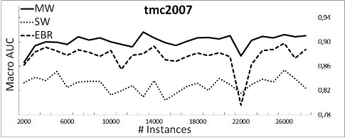
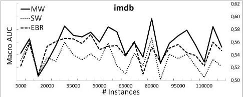
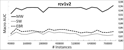
Table 3 reports the results on the threshold-dependent macro-averaged F1 measure for all datasets. For each method, the two columns show the performance with and without thresholding.
We first notice that all three methods have substantial gains in macro-averaged F1 when the thresholding technique is utilized. This shows that the proposed thresholding technique works quite well and at the same time stresses the importance of using a proper thresholding strategy for multi-label classification of data streams.
Next, we note that MW is better than its competitors in macro-averaged F1 in all datasets, both with and without thresholding, except in one case. The exception is rcv1v2, where MW without thresholding is worse than SW. This stresses even more the importance of a proper thresholding strategy, given that in rcv1v2 the AUC of MWwas far better than SW (and EBR). Using thresholding, MW achieves the best result in all datasets. This shows again that the multiple windows approach can also work well when bipartitions are required as output, provided it is coupled with an appropriate thresholding strategy.
| MW | SW | EBR | ||||
|---|---|---|---|---|---|---|
| Dataset | no | th | no | th | no | th |
| tmc2007 | 0.415 | 0.516* | 0.313 | 0.460 | 0.177 | 0.461 |
| imdb | 0.115 | 0.131* | 0.040 | 0.116 | 0.004 | 0.103 |
| rcv1v2 | 0.228 | 0.401* | 0.299 | 0.323 | 0.071 | 0.268 |
In a second set of experiments (not reported here due to space limitations), we have given more examples to the methods. We observed that the performance increased, especially for tmc2007 and imdb. We suspect that this is due to the rather static nature of these datasets, where it is intuitive that giving more examples for training increases the predictive performance. The improvement was only minor for rcv1v2, which is a more dynamic dataset and simulates better an evolving multi-label stream.
5 Conclusions and FutureWork
We presented a novel method for multi-label stream classification which adopts a multiple windows approach to deal with concept drift and skewness in the distribution of positive and negative examples of each label. Our method, being independent of the base classifier, offers a general framework for dealing with evolving multi-label streams. Space and time efficient implementations of this method were discussed. We also proposed a batch-incremental thresholding technique which aims to further reduce the impact of class imbalance to the learning process.
The empirical evaluation showed that 1) the theoretical advantage of our learning method is verified in practice by substantial gains in threshold-independent evaluation and 2) our thresholding technique is able to effectively adjust the decision thresholds, again with significant gains in predictive accuracy for all methods studied.
In the future we plan to 1) give our method the ability to model label correlations by utilizing methods like [Read et al., 2009], 2) dynamically adjust the size of the positive window of each label using a drift detection method, 3) employ a mechanism to efficiently deal with label set expansion, 4) experiment with different binary base classifiers and 5) evaluate our method in synthetic datasets modeling various concept drift patterns and imbalance degrees.
@inproceedings{ijcai2011p266,
  title     = {Dealing with Concept Drift and Class Imbalance in Multi-Label Stream Classification},
  author    = {Xioufis, Eleftherios Spyromitros and Spiliopoulou, Myra and Tsoumakas, Grigorios and Vlahavas, Ioannis P.},
  booktitle = {Proceedings of the Twenty-Second International Joint Conference on
               Artificial Intelligence, {IJCAI-11}},
  publisher = {AAAI Press/International Joint Conferences on Artificial Intelligence},
  editor    = {Toby Walsh},
  pages     = {1583--1587},
  year      = {2011},
  month     = {7},
  doi       = {10.5591/978-1-57735-516-8/IJCAI11-266},
  url       = {https://doi.org/10.5591/978-1-57735-516-8/IJCAI11-266},
}
TY - CPAPER TI - Dealing with Concept Drift and Class Imbalance in Multi-Label Stream Classification AU - Xioufis, Eleftherios Spyromitros AU - Spiliopoulou, Myra AU - Tsoumakas, Grigorios AU - Vlahavas, Ioannis P. T2 - Proceedings of the Twenty-Second International Joint Conference on Artificial Intelligence, IJCAI-11 PB - AAAI Press/International Joint Conferences on Artificial Intelligence PY - 2011 SP - 1583 EP - 1587 DO - 10.5591/978-1-57735-516-8/IJCAI11-266 UR - https://doi.org/10.5591/978-1-57735-516-8/IJCAI11-266 ER -Copied
Machine-readable versions of this paper, for tools and AI agents:





