
Angular Decomposition
Proceedings of the Twenty-Second International Joint Conference on Artificial Intelligence. Pages 1505-1509.
https://doi.org/10.5591/978-1-57735-516-8/IJCAI11-253
© 2011 International Joint Conferences on Artificial Intelligence
Abstract
Dimensionality reduction plays a vital role in pattern recognition. However, for normalized vector data, existing methods do not utilize the fact that the data is normalized. In this paper, we propose to employ an Angular Decomposition of the normalized vector data which corresponds to embedding them on a unit surface. On graph data for similarity/kernel matrices with constant diagonal elements, we propose the Angular Decomposition of the similarity matrices which corresponds to embedding objects on a unit sphere. In these angular embeddings, the Euclidean distance is equivalent to the cosine similarity. Thus data structures best described in the cosine similarity and data structures best captured by the Euclidean distance can both be effectively detected in our angular embedding. We provide the theoretical analysis, derive the computational algorithm, and evaluate the angular embedding on several datasets. Experiments on data clustering demonstrate that our method can provide a more discriminative subspace.
- [Belkin and Niyogi, 2003] M. Belkin and P. Niyogi. Lapla- cian eigenmaps for dimensionality reduction and data rep- resentation. Neural Computation, 15(6):1373-1396, 2003.
- [Ding and He, 2004] C. Ding and X. He. K-means clustering via principal component analysis. In Int'l Conf. Machine Learning (ICML), 2004.
- [Duda et al., 2001] R.O. Duda, P.E. Hart, and D.G. Stork. Pattern Classification (2nd ed). Wiley Interscience, New York, 2001.
- [Genton et al., 2001] M.G. Genton, N. Cristianini, J.S. Tay- lor, and R. Williamson. Classes of kernels for machine learning: a statistics perspective. Journal of Machine Learning Research, 2:299-312, 2001.
- [Hall, 1971] K. M. Hall. R-dimensional quadratic placement algorithm. Management Science, 17:219-229, 1971.
- [He and Niyogi, 2003] X. He and P. Niyogi. Locality pre- serving projections. In NIPS 2003, 2003.
- [Luo et al., 2009] D. Luo, C. Ding, H. Huang, and T. Li. Non-negative laplacian embedding. In ICDM, pages 337- 346, 2009.
- [Roweis and Saul, 2000] S.T. Roweis and L.K. Saul. Nonlin- ear dimensionality reduction by locally linear embedding. Science, 290(22):2323-2326, 2000.
- [Tenenbaum et al., 2000] J.B. Tenenbaum, V.de. Silva, and J.C. Langford. A global geometric framework for nonlin- ear dimensionality. Science, 290(22):2319-2323, 2000.
- [Wang et al., 2010] H. Wang, C. Ding, and H. Huang. Multi- label linear discriminant analysis. In ECCV, pages 126- 139, 2010.
- [Yan et al., 2007] S. Yan, D. Xu, B. Zhang, H. Zhang, Q. Yang, and S. Lin. Graph embedding and extensions: a general framework for dimensionality reduction. IEEE Trans. Pattern Anal. Mach. Intellig, 29(1):40-51, 2007.
- [Zhang and Zha, 2004] Z. Zhang and Z. Zha. Principal man- ifolds and nonlinear dimensionality reduction via tangent space alignment. SIAM J. Scientific Computing, 26:313- 338, 2004.
References were extracted automatically from the PDF and may contain errors.
Full text extracted automatically from the PDF; figures, tables and equations may differ. The PDF is the version of record.
1 Introduction
Dimensionality reduction is an important problem in pattern recognition, and various methods have been proposed. From the point of view of data embedding, there are two categories of embedding approaches. For vector data embedding, Principal Component Analysis (PCA) for unsupervised data and Linear Discriminate Analysis (LDA)[Duda et al., 2001; Wang et al., 2010] for supervised data are the two most widely used linear algorithms because of their relative simplicity and effectiveness. For graph data embedding, Laplacian Embedding (LE) [Hall, 1971; Belkin and Niyogi, 2003; Luo et al., 2009] is a classical method; in addition, Manifold learning also is one important class of popular approaches such as Isomap [Tenenbaum et al., 2000], Locally Linear Embedding (LLE) [Roweis and Saul, 2000], Local Tangent Space Alignment (LTSA)[Zhang and Zha, 2004], Locality Preserving Projections[He and Niyogi, 2003], etc.
The most widely used PCA projects data into a subspace using a least square data representation error function. However, in many applications such as information retrieval, image analysis, and genomics, normalized vector data come naturally. PCA does not take advantage of this special nature for the normalized data. Furthermore, in machine learning, many graph data including pairwise similarities are produced by kernel functions [Genton et al., 2001], such as the most widely used RBF kernel, which usually have constant/unit diagonal elements. Most existing embedding methods do not utilize this property.
This motivate us to propose a new embedding method called Angular Decomposition (also called angular embedding) to deal with normalized data or graphs/kernels with constant diagonal elements. The decompositions correspond to embedding data onto a low-dimensional spherical surface. Although Angular Decomposition is best suited to normalized vector data and graph data with constant diagonal elements, it also applies to un-normalized data or graph data with non-constant diagonal. One important feature of angular embedding is that because the embedded data are on the unit sphere, the cosine similarity is equivalent to the Euclidean distance. Thus data structures best described in the cosine similarity and data structures best captured by the Euclidean distance can both be effectively detected in our angular embedding.
Below, we first introduce Angular Decomposition for vector data and Angular Decomposition for graph data. We then derive computational algorithms for each decomposition respectively. We evaluate these new data decompositions for unsupervised learning. We perform angular embedding on several common datasets. Experiment results demonstrate the effectiveness of these new decompositions as compared to existing approaches.
2 Angular Decomposition
We start with a brief discussion of PCA, which is the most widely used dimensionality reduction method. Let the input data matrix X = (x1, · · · , xn) ∈ ℜp×n contains the collection of n data column vectors in p dimension space. In image processing, each column xi is a linearized array of pixels' gray levels; in text processing, xi is a document. PCA finds the optimal low-dimensional (k-dim) subspace defined (spanned) by the principal directions U = (u1, · · · , uk) ∈ ℜp×k . The projected data points in the new subspace are V = (v1, · · · , vn) ∈ ℜk×n. PCA finds U and V by minimizing
The global optimal solution is the rank-k singular value decomposition, X ≈ UΣV . We absorb Σ into V in Eq(1).
2.1 Angular Decomposition of vector data
Our primary focus is the normalized vector data, i.e., ‖xi‖2 = 1, i = 1, · · · , n. Here for simplicity, we assume data are normalized into unit length. We note that many data came naturally normalized. Our starting point is that PCA is not specifically designed to work on normalized vector data, i.e., in general, the projection in the PCA subspace ‖vi‖2 ̸= 1. Although we can show
This means that for normalized data, the projection (in the PCA subspace) vi is not normalized, but is approximately normalized if the subspace dimension k is sufficiently large.
To fully take advantage of the special nature of the normalized data, we propose the following Angular Decomposition
where I is the identical matrix.
One improvement can be made. Because the ranks of U, V are low, we introduce an overall scale α to improve the data representation. Furthermore, to distinguish the normalized variable, we use H instead of V as
Please note we use the transposition H T following convention. Thus the final Angular Decomposition is defined as
Note that (HH T )ii = ‖hi‖2 is the length of embedding vector.
The most important advantage of Angular Decomposition is that in the embedding space, the (k -1) dimension sphere, the Euclidean distance is equivalent to the cosine similarity:
Theorem1: InAngular Decomposition, the Euclidean distance is equivalent to the cosine similarity.
Proof: The cosine similarity for vector hi and hj is defined as cos θ(hi, hj) = hi · hj/‖hi‖‖hi‖. The Euclidean distance between vectors hi and hj is
where ‖hi‖ = 1 in our Angular Decomposition. Furthermore, large dij corresponds to small cos θ(hi, hj). Thus Euclidean distance is equivalent to cosine similarity. QED
This equivalence is useful because the Euclidean distance captures some intrinsic properties for some datasets while the cosine similarity captures the essential properties for some other datasets. It makes the angular embedding to be a more suitable low-dimensional embedding of vector data.
The computational algorithm will be given in Section 3.1. Here we note that the algorithm updates α, U, H one at a time; and each of them is computed from a closed-form optimal solution.
2.2 Angular Decomposition for Graph Data
In many applications, the input data are pairwise similarities which are generally viewed as edge weights between nodes of an undirected graph [Yan et al., 2007]. We wish to embed the graph data. Most graph data are pairwise similarity matrices Sij that describe similarity between objects i and j.
Consider the linear kernel (the Gram matrix) constructed from the normalized vector data above. The similarity between i, j is
Note that Sii = 1 for i = 1 · · · n.
Additionally, many kernel functions such as RBF kernel have unit diagonal elements: Kii = 1, i = 1 · · · n.
For any positive semi-definite (p.s.d.) kernel matrix K (rank(K)= r), it can be exactly embedded in full rdimensional space using the r eigenvectors. Based on spectral expansion, the full space (r-dimensional space) embedding of object i is
where vl(i) is the i-th element of eigenvector vl, l = 1 · · · r. Define the dissimilarity between i, j as
We have
Theorem 2: For any p.s.d. kernel matrix K with Kii = 1, their dissimilarity can be expressed exactly as
Furthermore, the embedding is unit-normalized: ‖zi‖ = 1. Proof: A p.s.d. kernel has a spectral expansion
proving Eq.(8). From the definition of zi, we have
In real application, embedding to low-dimensional space is useful because it reveal the inherent structure of the data. Thus we embed the kernel matrix in a k-dimensional space where k is in general close to the number of distinct clusters, which is much smaller than r. Therefore, for any kernel matrix K, we have
because zi = (Zi1, · · · , Zik)T , thus ‖zi‖2 = ∑kl=1 Z 2 il = (ZZ T )ii = 1 retains the unit-normalization property. Intuitively, our Angular Decomposition is very natural since both K and ZZ T have identical diagonal elements.
In this paper, we view graph data, the similarity matrix S, as from a kernel with unit diagonal elements. By introducing α to compensate the fact that the embedding space dimension is k which is far less than rank(S), the final Angular Decomposition is defined as,
The computational algorithm is given in Section 3.2.
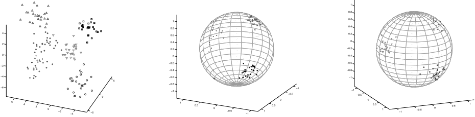
Figure 1 shows the synthetic data points which contain 6 clusters and corresponding Angular Decomposition Embedding result. With Angular Decomposition, the data structures and distributions are generally more apparent. We will show in experiments that our methods also achieve better results.
2.3 Brute-force Angular Embedding (BAE)
We note that for embedding data on spherical surface can be done in a brute-force (naive) way: simply normalize the embedding vectors H. More specifically, this consists of two steps. For vector data, we (1) compute the low-dimensional represents V via SVD(X) = UΣV T , and (2) normalize each column of ΣV T to unit length as the final embedding vector. For graph data, we also (1) compute eigenvectors of similarity matrix as S = VΣV T and (2) normalize embedding coordinates rows of V Σ1/2 to unit length.
The experiments in Section 4 will demonstrate that compared to the brute-force approaches, our more vigorous approaches of Eq.(4) and (11) provide embedding coordinates which (a) are better data representation/approximation (in the same sense that PCA is a data representation/approximation method too), (b) provide better machine learning results such as clustering accuracy .
3 Algorithms and analysis
Here we provide algorithms and accompanying analysis for the two Angular Decomposition methods presented above.
3.1 Angular Decomposition of vector data
We optimize the objective function of Eq.(4) via an iterative updating algorithm that alternatively updates α, H, and U one at a time. We give the closed-form solution for each of them explicitly. The algorithm starts with initialization of U, H.
Step (V0). Initialization.
Compute first k terms of SVD(X) = UΣV T . Set U0 = U, H0 = V Σ.
We then update α,H, U one at a time in Steps (V1 - V3). They are repeated until convergence.
Step (V1). Compute α while fixing U and H.
From Eq.(4), the optimal solution for α is given by
Proof we write the objective function of Eq.(4) as
since U T U = I and (HH T )ii = 1.
For variable α, the optimization is unrestricted. We set gradient to zero
and obtain the optimal solution in Eq.(12). QED.
Step V2: Compute H while fixing α and U .
We update H using the following:
Lemma 1. Given fixed α and U in Eq.(4), the optimization for H in Eq.(4) has close form solution:
Proof. This is an optimization with equality constraints. We use Lagrangian multiplier method, where the λi is the Lagrangian multiplier to the condition function (H T H)ii = 1. From Eq.(13), the Lagrangian function is
Setting the derivatives of the Lagrangian function to zero,
we obtain
Now, we need to find the values of the Lagrangian multipliers. Multiply Hij and sum over j for above equation we have:
This gives the values of Lagrangian multipliers:
Substituting this into Eq.(15), we obtain Eq.(14). QED
Step V3: Update U while fixing α, H.
We compute U using the following:
Lemma 2. Given fixed α and H in Eq.(4), the optimization for U in Eq.(4) has close-form solution:
where A, B are obtained from the singular value decomposition of the p-by-k matrix XH:
where A ∈ ℜp×k contains the left singular vectors and B ∈ ℜk×k contains the right singular vectors. Without loss of generality, we assume p ≥ k.
Proof. From the last equation of Eq.(13), the minimization of J2(U) becomes
Substituting XH = AΣBT fromEq.(14), this becomes
We now prove that U ∗ = ABT is the optimal solution.
The proof is complete if we can prove that tr(Σ) is an upper bound of J(U): for any feasible solution U, we have
With this, U ∗ = ABT is a global optimal solution because J(U ∗ ) = tr(Σ) reaches the upper bound and therefore no other solution has better objective function value.
To prove the upper bound Eq.(20), we prove that every element of matrix (BT U T A) is less than 1, i.e.,
because if this is the case, we have
proving the upper bound Eq.(20).
To prove the inequality of Eq.(21), we note that there exits the complement space A⊥ ∈ ℜp×(p-k) such that matrix [A,A⊥] forms a complete basis: [A,A⊥]T [A,A⊥] = [A, A⊥][A, A⊥]T = I. Thus we have (BT U T [A, A⊥])(BT U T [A, A⊥])T = BT U T UB = BT B = I.
This implies for any s, 1 ≤ s ≤ k, we have
implying the inequality of Eq.(21) must be true. QED.
3.2 Angular Decomposition of graph data
We provide the algorithm for computing the Angular Decomposition for an input graph data S (the similarity matrix) using Eq.(11). The embedding coordinates on the sphere are computed via an iterative updating algorithm that alternatively updates α, H, λ one at a time, where λ are Lagrangian multipliers for enforcing the constraints when we update H according to Eq.(11). Step (G0) is the initialization. Steps (G1 - G3) update α, H, λ and are repeated until convergence.
Step (G0). Initialization.
Compute first k terms of eigen-decomposition S = V ΣV T . Set H0 = V Σ 1 2 .
We update α,H, λ alternately one at a time where λ are Lagrangian multipliers for enforcing the constraints when we update H according to Eq.(11) until convergence.
Step (G1): Update α while fix H
We update parameter α using this formula:
Proof. Setting the gradient of J4 of Eq.(11) to zero,
we obtain optimal α∗ in Eq.(22). QED.
Step (G2): Update Lagrangian multipliers λ while fixing α, H.
When updating H according to Eq (11), we use Lagrangian multipliers {λi} to enforce the constraints, (HH T )ii = 1.
We compute λi using the following rule:
Proof: This is derived from the KKT condition for constrained optimization. The Lagrangian function of J4 is
Setting the derivatives to zero, we have
Multiply Hij and sum over j, we obtain
Using the constraint (HH T )ii = 1, we obtain λi as Eq.(23).
Step (G3): Update H while fixing α and λ
We update H using gradient descent method,
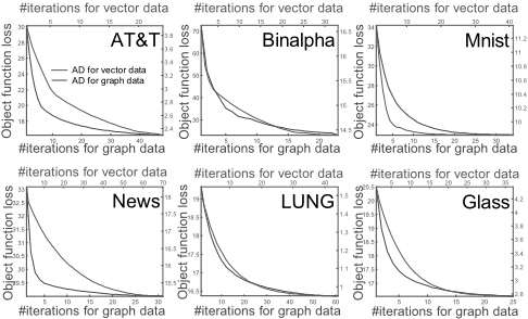
where parameter η adjusts the stepsize the solution goes along the negative gradient direction while the Lagrangian multiplier term enforces the solution on unit sphere. We typically set η = 0.01 (∑ij |Hij|) / (∑ij | ∂L(H) ∂Hij |) . The convergence is demonstrated in experiments (see Fig.2).
4 Experiments
We apply Angular Decomposition on six real-world datasets, including vector data and graph data.
4.1 Datasets Description
The method is tested on six datasets, involving three available image datasets, one textual dataset, one genomic dataset and one physical dataset.
AT&T Faces Dataset contains ten different images of each 40 distinct persons and the size of each image is 92×112 pixels, with 256 grey levels per pixel. In our experiment, each face image was resized into 32×32 and reshaped into a vector of 1024 dimension.
Binary Alphabet Dataset contains 26 handwritten alphabets A∼Z. Each sample is a 20 × 16 binary image. We select 30 images for every alphabet and reshape each image into one vector of 320 dimension.
MNIST Hand-written Digit Dataset is consisted of 8-bit gray-scale images of digits from "0"to "9", about 6000 examples of each class (digit). Each image is centered on a 28 ×28 grid. Here, we randomly choose 100 images from each digit, and convert them to vectors of 784 dimension.
Twenty Newsgroups Dataset is a collection of approximately 20,000 message documents, partitioned evenly across 20 different newsgroups. Each message is described by binary data of 100 words. Here, one hundred messages from each of the twenty newsgroups were chosen at random and converted to a binary vector.
LUNG Dataset contains in total 203 samples in five classes. Each sample has 12600 genes. We removed the genes with standard deviations smaller than 50 expression units, and then obtained a data set with 3312 genes.
Glass Identification Dataset describes main characteristics of the glass dataset and its attributes. It is consisted of 214 observation containing examples of the chemical analysis of 7 different types of glass. Every sample has 9 features.
The data from above datasets are vector data. To convert them into graph data, the similarity matrix Sij, we choose RBF kernel Sij = e-γ‖xi-xj‖2 , where γ = 0.7/d2, d = ∑ij ‖xi - xj‖/n(n - 1).
4.2 Algorithm convergence
We first show the convergence of the proposed algorithms on the six datasets. The results are shown in Figure 2. The algorithms converge after around 50 iterations.
4.3 Data Reconstruction
We compare the data representation/reconstruction capability of Angular Decomposition (hereinafter "AD") with the brute-force angular embedding (BAE, see §2). We compute the residual of data representation in Eqs.(4)and (11) and the corresponding residual for BAE for the two kinds of data.
For vector data, the residual for BAE is computed by choosing β that minimizes the object function,
where Q is obtained from the normalized embedding coordinate directly as described in §2.3. For graph data, the residual for BAE objective function is computed by optimizing β that minimizes
| BAE for vector data | AD for vector data | BAE for graph data | AD for graph data | |
|---|---|---|---|---|
| AT&T | 3.949 | 2.302 | 17.396 | 16.612 |
| BinAlp | 16.579 | 14.183 | 24.060 | 23.026 |
| Mnist | 10.328 | 9.583 | 24.590 | 22.869 |
| News | 18.664 | 15.110 | 34.023 | 29.012 |
| Lung | 1.887 | 0.956 | 18.600 | 16.429 |
| Glass | 4.206 | 2.798 | 14.210 | 12.643 |
The obtained residual results are shown in Table 1 for six datasets. These results show that AD has consistently lower residual than BAE in all cases. This indicates our vigorous approach is more effective in preserving the structure of data.
4.4 Clustering
We evaluate the unsupervised learning on Angular Decomposition. We use Angular Decomposition to embed vector data and graph data on the unit sphere, and then perform the Kmeans clustering on these embedding coordinates. For comparison purposes, we also show clustering results on the original high-dimensional data X and the PCA projection data. Additionally, we use BAE do subspace embedding for vector data and graph data (with the same parameters as our Angular Decomposition) and run clustering on the embedded data. To get robust statistics, we run K-means 50 times using different random starts and computed the average as the final results.
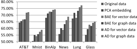
Clustering accuracy measures the percentage of data points correctly clustered. It is obtained by first computing the confusion matrix. The Hungarian algorithm is then used to permutate columns of confusion matrix to maximize the sum of the diagonal elements, which is the clustering accuracy.
Results of clustering on the six datasets are shown in Figure 2. Six different methods are compared and shown in Fig.2. From the experimental results, we observed the following:
(F1) Embedding into low-dimensional subspace improves the performance. On all six datasets, for both vector data and graph data, using either BAE or AD, the K-means clustering results are better than in original high-dimensional data. That PCA embedding improves K-means clustering is analyzed in [Ding and He, 2004]; the improvements for graph embedding can be viewed as kernel PCA improves kernel K-means clustering [Ding and He, 2004].
(F2) Graph data produces better results than the vector data for the same dataset. This is consistent on all six datasets. It is likely due to the flexibility of graph representation, as compared to K-means clustering in vector space with a objective function that favors ball-shaped clusters.
(F3) AD perform consistently better than BAE.
5 Conclusions
Angular Decomposition embeds high-dimensional data into a low-dimensional spherical space. This takes advantage of the special nature of the normalized data and integrating the cosine similarity and the Euclidean distance at the same time, and yields a more discriminative subspace for highdimensional data. Two efficient algorithms are developed to solve the proposed Angular Decomposition problems for vector data and graph data respectively. Extensive experiments on six real datasets show that angular embedding is more effective to exhibit class structures than other related methods. The experiments almost show that (1) clustering in lowdimensional embedding space consistently outperform those in original high dimensional data and (2) Using graph data gives better results than using vector data.
Acknowledgment
The research of D.Sun, J.Tang, B.Luo are supported by the NSFC 61073116, 61003038,61003131. C.Ding is supported by NSF-CCF-0830780, NSF-DMS-0915228, NSFCCF-0917274.
@inproceedings{ijcai2011p253,
  title     = {Angular Decomposition},
  author    = {Sun, Dengdi and Ding, Chris H. Q. and Luo, Bin and Tang, Jin},
  booktitle = {Proceedings of the Twenty-Second International Joint Conference on
               Artificial Intelligence, {IJCAI-11}},
  publisher = {AAAI Press/International Joint Conferences on Artificial Intelligence},
  editor    = {Toby Walsh},
  pages     = {1505--1509},
  year      = {2011},
  month     = {7},
  doi       = {10.5591/978-1-57735-516-8/IJCAI11-253},
  url       = {https://doi.org/10.5591/978-1-57735-516-8/IJCAI11-253},
}
TY - CPAPER TI - Angular Decomposition AU - Sun, Dengdi AU - Ding, Chris H. Q. AU - Luo, Bin AU - Tang, Jin T2 - Proceedings of the Twenty-Second International Joint Conference on Artificial Intelligence, IJCAI-11 PB - AAAI Press/International Joint Conferences on Artificial Intelligence PY - 2011 SP - 1505 EP - 1509 DO - 10.5591/978-1-57735-516-8/IJCAI11-253 UR - https://doi.org/10.5591/978-1-57735-516-8/IJCAI11-253 ER -Copied
Machine-readable versions of this paper, for tools and AI agents:





