
Robust Principal Component Analysis with Non-Greedy l1-Norm Maximization
Proceedings of the Twenty-Second International Joint Conference on Artificial Intelligence. Pages 1433-1437.
https://doi.org/10.5591/978-1-57735-516-8/IJCAI11-242
© 2011 International Joint Conferences on Artificial Intelligence
Abstract
Principal Component Analysis (PCA) is one of the most important methods to handle high-dimensional data. However, the high computa-tional complexity makes it hard to apply to the large scale data with high dimensionality, and the used 2-norm makes it sensitive to outliers. A recent work proposed principal component analysis based on 1-norm maximization, which is efficient and robust to outliers. In that work, a greedy strategy was applied due to the difficulty of directly solving the 1-norm maximization problem, which is easy to get stuck in local solution. In this paper, we first propose an efficient optimization algorithm to solve a general 1-norm maximization problem, and then propose a robust principal component analysis with non-greedy 1-norm maximization. Experimental results on real world datasets show that the non-greedy method always obtains much better solution than that of the greedy method.
- [Aanas et al., 2002] H. Aanas, R. Fisker, K. Astrom, and J.M. Carstensen. Robust factorization. IEEE Transactions on PAMI, 24(9):1215-1225, 2002.
- [Baccini et al., 1996] A. Baccini, P. Besse, and A. de Faguerolles. A L1-norm PCA and heuristic approach. In Proceedings of the International Conference on Ordinal and Symbolic Data Analy- sis, volume 1, pages 359-368, 1996.
- [Boyd and Vandenberghe, 2004] S.P. Boyd and L. Vandenberghe. Convex optimization. Cambridge University Press, 2004.
- [De La Torre and Black, 2003] F. De La Torre and M.J. Black. A framework for robust subspace learning. International Journal of Computer Vision, 54(1):117-142, 2003.
- [Ding et al., 2006] Chris H. Q. Ding, Ding Zhou, Xiaofeng He, and Hongyuan Zha. R1-PCA: rotational invariant L1-norm principal component analysis for robust subspace factorization. In ICML, pages 281-288, 2006.
- [Donoho, 2006] David L. Donoho. Compressed sensing. IEEE Transactions on Information Theory, 52(4):1289-1306, 2006.
- [Galpin and Hawkins, 1987] J.S. Galpin and D.M. Hawkins. Meth- ods of L1 estimation of a covariance matrix. Computational Statistics & Data Analysis, 5(4):305-319, 1987.
- [Huang and Ding, 2008] Heng Huang and Chris H. Q. Ding. Ro- bust tensor factorization using r1 norm. In CVPR, 2008.
- [Ke and Kanade, 2005] Q. Ke and T. Kanade. Robust L1 norm fac- torization in the presence of outliers and missing data by alterna- tive convex programming. In CVPR, pages 739-746, 2005.
- [Kwak, 2008] N. Kwak. Principal component analysis based on L1- norm maximization. IEEE Transactions on PAMI, 30(9):1672- 1680, 2008.
- [Lathauwer, 1997] Lieven De Lathauwer. Signal Processing based on Multilinear Algebra. PhD thesis, Faculteit der Toegepaste Wetenschappen. Katholieke Universiteit Leuven, 1997.
- [Li et al., 2010] Xuelong Li, Yanwei Pang, and Yuan Yuan. L1- norm-based 2DPCA. IEEE Transactions on Systems, Man, and Cybernetics, Part B, 38(4), 2010.
- [Liu et al., 2010] Yang Liu, Yan Liu, and Keith C. C. Chan. Mul- tilinear maximum distance embedding via l1-norm optimization. In AAAI, 2010.
- [Nie et al., 2010a] Feiping Nie, Heng Huang, Xiao Cai, and Chris Ding. Efficient and robust feature selection via joint ℓ2,1-norms minimization. In NIPS, 2010.
- [Nie et al., 2010b] Feiping Nie, Dong Xu, Ivor Wai-Hung Tsang, and Changshui Zhang. Flexible manifold embedding: A frame- work for semi-supervised and unsupervised dimension reduc- tion. IEEE Transactions on Image Processing, 19(7):1921-1932, 2010.
- [Pang et al., 2010] Yanwei Pang, Xuelong Li, and Yuan Yuan. Ro- bust tensor analysis with L1-norm. IEEE Transactions on Cir- cuits and Systems for Video Technology, 20(2):172-178, 2010.
- [Schölkopf et al., 1998] Bernhard Schölkopf, Alex J. Smola, and Klaus-Robert Müller. Nonlinear component analysis as a ker- nel eigenvalue problem. Neural Computation, 10(5):1299-1319, 1998.
- [Wright et al., 2009] J. Wright, A. Ganesh, S. Rao, and Y. Ma. Ro- bust principal component analysis: Exact recovery of corrupted low-rank matrices via convex optimization. NIPS, 2009.
- [Xiang et al., 2008] Shiming Xiang, Feiping Nie, and Changshui Zhang. Learning a mahalanobis distance metric for data cluster- ing and classification. Pattern Recognition, 41(12):3600-3612, 2008.
- [Yang et al., 2009] Yi Yang, Yueting Zhuang, Dong Xu, Yunhe Pan, Dacheng Tao, and Stephen J. Maybank. Retrieval based interac- tive cartoon synthesis via unsupervised bi-distance metric learn- ing. In ACM Multimedia, pages 311-320, 2009.
- [Zhang et al., 2010] Changshui Zhang, Feiping Nie, and Shiming Xiang. A general kernelization framework for learning algo- rithms based on kernel PCA. Neurocomputing, 73(4-6):959-967, 2010.
References were extracted automatically from the PDF and may contain errors.
Full text extracted automatically from the PDF; figures, tables and equations may differ. The PDF is the version of record.
1 Introduction
In many real-world applications such as face recognition and text categorization, the dimensionality of data are usually very high. Directly handle the high-dimensional data is computationally expensive and at the same time the performance could be very poor because the number of available data is always limited and the noise in the data would increase dramatically as the dimensionality increases. Dimensionality reduction or distance metric learning is one of the most important and effective methods to handle highdimensional data [Xiang et al., 2008; Yang et al., 2009; Nie et al., 2010b]. Among the dimensionality reduction methods, Principal Component Analysis (PCA) is one of the most widely applied methods due to its simplicity and effectiveness. Given a dataset, PCA finds a projection matrix to maximize the variance of the projected data points under this projection matrix, and the structure of original data could be effectively preserved under the projection.
∗This research was funded by US NSF CCF-0830780, 0939187, 0917274, NSF DMS-0915228, NSF CNS-0923494, 1035913.
In the past decades, the traditional PCA has been successfully applied in many problems. However, it has several drawbacks. First, it has to performSingular Vector Decomposition (SVD) on input data matrix or eigen-decomposition on covariance matrix, which is computationally expensive and difficult to apply when both the number of data and the dimensionality are very high. Second, it is sensitive to outliers because it is intrinsically based on ℓ2-norm and the outliers with large norm can be exaggerated by using the ℓ2norm. Many works [Baccini et al., 1996; Aanas et al., 2002; De La Torre and Black, 2003; Ke and Kanade, 2005; Ding et al., 2006; Wright et al., 2009] have devoted effort to alleviate this problem and improve the robustness to outliers. [Baccini et al., 1996; Ke and Kanade, 2005] consider the problem of finding a subspace such that the sum of ℓ1-norm distances of data points to the subspace is minimized. Although the robustness to outliers is improved by this method, it is computationally expensive and more importantly, the used ℓ1-norm is not invariant to rotation and the performance usually very poor when applied to K-means clustering [Ding et al., 2006]. To solve this problem, R1-PCA was proposed which is invariant to rotation and demonstrated favorable performance [Ding et al., 2006]. However, R1-PCA iteratively performs the subspace iteration algorithm in the high-dimensional original space, which is computationally expensive. The extension of R1-PCA to tensor version can be found in [Huang and Ding, 2008].
Recently, a robust principal component analysis based on ℓ1-norm maximization is proposed in [Kwak, 2008], and a similar work can be found in [Galpin and Hawkins, 1987]. This method is invariant to rotation and is also robust to outliers. In [Kwak, 2008], an efficient algorithm is proposed to solve the ℓ1-norm maximization problem. The algorithm only need to perform matrix-vector multiplication, and thus can be applied in the case that both the number of data and the dimensionality are very high. Some works on its tensor version and supervised version can be found in [Li et al., 2010; Liu et al., 2010; Pang et al., 2010]. Due to the difficulty of directly solving the ℓ1-normmaximization problem, all these works use a greedy strategy to solve it. Specifically, the projection directions are sequentially optimized one by one. This kind of greedy method is easy to get stuck in a local solution.
In this paper, we focus on solving the ℓ1-norm maximization problem. We first propose an efficient optimization algorithm to solve a general ℓ1-norm maximization problem. Theoretical analysis guarantees the algorithm will converge and usually converge to a local solution. The ℓ1-norm maximization problem in [Kwak, 2008] is a special case of the general problem, and thus the proposed optimization algorithm can be used to solve it directly in a non-greedy strategy. That is, all the projection directions can be optimized simultaneously. Experimental results on real datasets show that the non-greedy method always obtains much better solution than that of the greedy method.
The rest of this paper is organized as follows: We give a brief review of the work [Kwak, 2008] in §2. In §3, we propose an efficient algorithm to solve a general ℓ1-norm maximization problem and give theoretical analysis on it. Based on the algorithm, we solve the problem for the principal component analysis with greedy ℓ1-norm maximization in §4 and propose a principal component analysis with non-greedy ℓ1norm maximization in §5. In §6, we present experiments to verify the effectiveness of the proposed method. Finally, we draw the conclusions in §7.
2 Related work
Suppose the given data are X = [x1, x2, · · · , xn] ∈ Rd×n, where n and d are the number and the dimensionality of data points respectively. Without loss of generality, the data {xi}ni=1 are assumed to be centralized, i.e., ∑ni=1 xi = 0.
Denote the projection matrix W = [w1,w2, · · · ,wm] ∈ Rd×m. Traditional PCA method maximizes the variance of data in the projected subspace, and to solve the following optimization problem:
where St = 1n XX T is the covariancematrix, I is the identity matrix and T r(·) is the trace operator of a matrix. Denote the ℓ1-norm and ℓ2-norm of a vector by ‖·‖1 and ‖·‖2 , respectively. The problem (1) can be reformulated as the following problem:
Motivated by this reformulation, a recent work [Kwak, 2008] proposed to maximize the ℓ1-norm instead of the ℓ2-norm in PCA, and thus the robustness to outliers is improved. Then the problem becomes:
Directly solving this problem is difficult, thus the author use a greedy strategy to solve it. Specifically, the m projection directions {w1, w2, ..., wm} are optimized one by one. The first projection direction w1 is optimized by solving the following problem:
After the (k - 1)-th projection direction wk-1 has been obtained, the data matrix X is transformed to X = X wk-1(wk-1)T X, and then the k-th projection direction wk is optimized by solving the following problem:
In this greedy method, the only problem needed to solve is the problem (5) for each k. The work in [Kwak, 2008] proposed an iterative algorithm to solve this problem. The detailed procedure is:
1) t = 1. Initialize wtk ∈ Rd such that ‖(wtk )‖2 = 1.
2) For each i, if (wtk )T xi < 0, αi =
-1 otherwise αi = 1.
4) Iteratively perform steps 2 and 3 until converges.
In order to guarantee the algorithm converges to a local maximum, the algorithm adds an additional judgement after convergence. If there exists i such that (wtk )T xi = 0, then let wtk = (wtk + △w)/‖wtk + △w‖2 and go to step 2, where △w is a small nonzero random vector. However, such operation might make the algorithm interminable (for example, suppose there is a data point x that exactly locates on the mean of the data set, then x will be zero after centralization, and thus (wt )T x is always zero for any wt ). Moreover, it is possible that there exists i such that (wtk )T xi = 0 at the global maximum. In this case, the algorithm can not have the chance to find the global maximum.
Subsequently, we will first propose an efficient algorithm to solve a general ℓ1-norm maximization problem. Based on it, we also solve the problem (5) for the principal component analysis with greedy ℓ1-norm maximization and propose the principal component analysis with non-greedy ℓ1-norm maximization by directly solve the problem (3). The additional judgement is not required in the new algorithms to obtain a local solution, and the non-greedy method always obtains much better solution than that of the greedy method in practice.
3 An efficient algorithm to solve a general ℓ1-norm maximization problem
Consider a general ℓ1-norm maximization problem as follows (we assume that the objective has an upper bound) :
where f(v) and gi(v) for each i are arbitrary functions, and v ∈ C is an arbitrary constraint. Although there are many methods to solve the ℓ1-norm minimization problem in compressed sensing and sparse learning [Donoho, 2006; Nie et al., 2010a], these methods can not be used to solve the ℓ1-norm maximization problem.
Rewriting the problem (6) as the following problem:
where αi = sgn(gi(v)), and sgn(·) is the sign function defined as follows: sgn(x) = 1 if x > 0, sgn(x) = -1 if x < 0, and sgn(x) = 0 if x = 0. Note that αi depends on v and thus is also a unknown variable. We propose an iterative algorithm to solve the problem (6), and prove that the proposed iterative algorithm will monotonically increase the objective of the problem (6) in each iteration, and will usually converge to a local solution.
The algorithm is described in Algorithm 1. In each iteration, αi is calculated by current solution v, and the solution v is updated with the current αi. The iterative procedure is repeated until the algorithm converges.
Algorithm 1: An efficient algorithm to solve a general ℓ1-norm maximization problem (6).
3.1 Theoretical analysis of the optimization algorithm
The convergence of the Algorithm 1 is demonstrated in the following theorem:
Theorem 1 The Algorithm 1 will monotonically increase the objective of the problem (6) in each iteration.
Proof: According to the step 2 in Algorithm 1, for each iteration t we have
For each i, note that αti = sgn(gi(vt )), so we have that ∣∣gi(vt+1 )∣∣ = sgn(gi(vt+1 ))gi(vt+1 ) ≥ sgn(gi(vt ))gi(vt+1 ) = αti gi(vt+1 ). Then ∣∣gi(vt+1 )∣∣ ≥ αti gi(vt+1 ) and note that |gi(vt )| - αti gi(vt ) = 0, we have:
Eq. (9) holds for every i, thus we have
Combining Eq. (8) and Eq. (10), we arrive at
Thus the Algorithm 1 will monotonically increase the objective of the problem (6) in each iteration t. □
As the objective of the problem (6) has an upper bound, Theorem 1 indicates that the Algorithm 1 will converge. The following theorem shows that the solution in the convergence will satisfy the KKT condition.
Theorem 2 The solution of the Algorithm 1 in the convergence will satisfy the KKT condition of the problem (6).
Proof: The Lagrangian function of the problem (6) is
where h(λ, v) is the Lagrangian term to encode the constraint v ∈ C in problem (6).
Taking the derivative 1 of L(v, λ) w.r.t v, and setting the derivative to zero, we have:
where αi = sgn(gi(v)).
Suppose the Algorithm 1 converges to a solution v∗ , from step 2 in Algorithm 1 we have
where α∗i = sgn(gi(v∗ )). According to the KKT condition [Boyd and Vandenberghe, 2004] of the problem in Eq. (14), we know that the solution v∗ satisfies Eq. (13), which is the KKT condition of the problem (6). □
In general, satisfying the KKT condition usually indicates that the solution is a local optimum solution. Theorem 2 indicates that the Algorithm 1 will usually converge to a local solution.
We can see that both the problem (5) and the problem (3) are the special cases of the problem (6), so we can use the proposed Algorithm 1 to solve these two problems. The key step of the Algorithm 1 is to solve the problem in step 2. In the next two sections, we give detailed derivation and algorithm to solve the problem (5) and the problem (3), respectively.
4 Principal component analysis with greedy ℓ1-norm maximization revisited
Recall that the principal component analysis with greedy ℓ1norm maximization only need to solve the following problem:
As described in Section 2, an algorithm proposed in [Kwak, 2008] can solve it. In this section, we solve it based on the Algorithm 1, and compare the differences between these two algorithms. According to the Algorithm 1, the key step to solve the problem (15) is to solve the following problem:
where αi = sgn((wt )T xi). Denote m = n∑ i=1 αixi, then we
can rewrite the problem (16) as
1 When x = 0, 0 is a subgradient of function |x|, so sgn(x) is the gradient or a subgradient of the function |x| in all the cases.
The Lagrangian function of the above problem is
Taking the derivative of L(w, λ) w.r.t w, and setting the derivative to zero, we have w = m/λ. Then λ = ‖m‖2 according to the constraint wT w = 1. So the optimal solution to the problem (16) is w = m/‖m‖2.
Based on the Algorithm 1, the algorithm to solve the principal component analysis with greedy ℓ1-norm maximization is described in Algorithm 2. We can see that the Algorithm 2 is almost the same as the one described in Section 2, except that the values of αi are different when (wtk )T xi = 0 and the Algorithm 2 does not have the additional judgement when the algorithm converges. When (wtk )T xi = 0, αi = 0 in Algorithm 2 while αi = 1 in the algorithm proposed in [Kwak, 2008]. Using the Algorithm 2 without the additional judgement, we can also obtain a local solution according to Theorem 2.
From Algorithm 2 we can see that the algorithm is efficient and only involves matrix-vector multiplication. The computational complexity is O(ndmt), where n, d,m is the number of data, dimension of original data and the dimension of the projected data respectively, and t is the iterative number. In practice, the algorithm usually converges in ten iterations. Therefore, the computational complexity of the algorithm is linear w.r.t both data number and data dimension, which indicates the algorithm is applicable in the case that both data number and data dimension are very high. If the data are sparse, the computational complexity is further reduced to O(nsmt), where s is the averaged number of non-zeros elements in a data point.
Algorithm 2: Principal component analysis with greedy ℓ1-norm maximization.
5 Principal component analysis with non-greedy ℓ1-norm maximization
The original problem in [Kwak, 2008] is to solve the following problem:
Algorithm 3: Principal component analysis with nongreedy ℓ1-norm maximization.
Since directly solving this problem is difficult, [Kwak, 2008] turns to solve it by a greedy method. In this paper, we propose a non-greedy method to directly solve the problem (19).
Based on the Algorithm 1, the key step to solve the problem (19) is to solve the following problem:
where the vectors αi = sgn((W t )T xi). Denote M = n∑ i=1 xiαTi , then we can rewrite the problem (20) as
Suppose the SVD of M is M = UΛV T , then Tr(W T M) can be rewritten as:
where Z = V T W T U, λii and zii are the (i, i)-th element of matrix λ and Z respectively.
Note that Z is an orthonormal matrix, i.e. Z T Z = I, so zii ≤ 1. On the other hand, λii ≥ 0 since λii is singular value of M. Therefore, Tr(W T M) = ∑i λiizii ≤ ∑i λii ,
and when zii = 1(1 ≤ i ≤ c), the equality holds. That is to say, Tr(W T M) reaches the maximumwhen Z = I. Recall that Z = V T W T U, thus the optimal solution to the problem Eq. (21) is
Based on the Algorithm 1, the algorithm to solve the principal component analysis with non-greedy ℓ1-norm maximization is described in Algorithm 3. According to Theorem 2, we can usually obtain a local solution.
From Algorithm 2 we can see that the algorithm is also efficient. Note that n ≫m in practice, thus the computational complexity of the algorithm is O(ndmt), which is the same as that of the greedy method. Similarly, the algorithm usually converges in ten iterations in practice. Therefore, the computational complexity of the algorithm is also linear w.r.t both data number and data dimension, which indicates the algorithm is applicable in the case that both data number and data dimension are very high. If the data are sparse, the computational complexity is further reduced to O(nsmt).
| Data set | Size | Dimensions | Classes |
|---|---|---|---|
| Jaffe | 213 | 1024 | 10 |
| Umist | 575 | 644 | 20 |
| Yale | 165 | 3456 | 15 |
| Coil20 | 1440 | 1024 | 20 |
| Palm | 2000 | 256 | 100 |
| USPS | 9298 | 256 | 10 |
5.1 Extensions to kernel and tensor cases
Similar to traditional PCA, the robust principal component analysis with ℓ1-norm maximization is also a linear method, and is difficult to handle data well with non-Gaussian distribution. A popular technique to deal with this problem is extending the linear method to kernel method. Obviously, the robust principal component analysis with ℓ1-norm maximization is invariant to rotation and shift, so this linear method satisfies the conditions in a generalized kernel framework in [Zhang et al., 2010], and thus can be kernelized using the framework. Specifically, the given data are transformed by KPCA [Sch¨olkopf et al., 1998], and then performAlgorithm 3 using the transformed data as input.
Another problem of the principal component analysis is that the method can only handle vector data. For 2D tensor or higher order tensor data, we have to vectorize the data to very high-dimensional vectors in order to apply this method. This approach will destroy the structural information of tensor data and also make the computational burden very heavy. A popular technique to deal with this problem is extending the vector method to tensor method. As the problem (19) of the principal component analysis with ℓ1-norm maximization only includes linear operator W T xi, it can be easily extended to the tensor method to handle tensor data directly. For simplicity, we only briefly discuss the case of 2D tensor, high order tensor cases can be readily extended by replacing the linear operator W T xi with tensor operator [Lathauwer, 1997]. Suppose the given data are X = [X1,X2, ...,Xn] ∈ Rr×c×n, where each data Xi ∈ Rr×c is a 2D tensor, n is the number of data points. Similarly, we assume that {Xi}ni=1 are centered, i.e., ∑ni=1 Xi = 0.
In the 2D tensor case, linear operator W T xi is replaced by U T XiV , where U ∈ Rr×r1 and V ∈ Rc×c1 are two projection matrices. Correspondingly, the problem (19) becomes:
As in other tensor method, problem (24) can be solved by alternative optimization technique (also named block coordinate descent). Specifically, when fixing U, the problem (24) reduced to the problem (19), and thus the V can be optimized by Algorithm 3. Similarly, U can also be optimized by Algorithm 3 when fixing V . The procedure is iteratively performed until converges.
6 Experiments
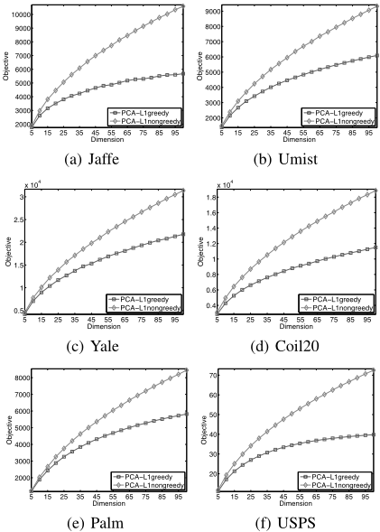
In this section, we present experiments to demonstrate the effectiveness of the proposed principal component analysis with non-greedy ℓ1-norm maximization (denoted by PCAℓ1nongreedy) compared to the greedy method (denoted by PCA-ℓ1greedy).
We use six image datasets from different domains to perform the experiments. A brief description of the datasets are shown in Table 1. In this experiment, we study the greedy and non-greedy optimization methods, and compare the objective values in Eq.(3) obtained by these two optimization methods.
In the first experiment, we run the greedy method and the non-greedy method with different projected dimensions m and the same initialization on each dataset. The projected dimensions varies from 5 to 100 with the interval 5. The results are shown in Figure 1. In the second experiment, we run the greedy method and the non-greedy method 50 times with the projected dimensions m = 50 on each dataset. In each time, the two methods use the same initialization. The results are shown in Table 2.
From Figure 1 and Table 2 we can see, the proposed nongreedy method obtains much higher objective values than that of the greedy method in all the cases. The results indicate that the proposed non-greedy method always obtains much better solution to the ℓ1-norm maximization problem (3) than the pervious greedy method.
| Data set | PCA-ℓ1greedy | PCA-ℓ1nongreedy | ||||||
|---|---|---|---|---|---|---|---|---|
| Min | Max | Min/Max | Mean | Min | Max | Min/Max | Mean | |
| Jaffe | 4722.86 | 4815.28 | 0.9808 | 4770.50 | 7349.87 | 7409.23 | 0.9920 | 7377.96 |
| Umist | 4649.03 | 4673.87 | 0.9947 | 4661.83 | 6316.97 | 6359.19 | 0.9934 | 6340.59 |
| Yale | 16058.68 | 16261.68 | 0.9875 | 16144.79 | 20964.16 | 21217.98 | 0.9880 | 21064.38 |
| Coil20 | 8753.97 | 8793.97 | 0.9955 | 8778.63 | 12860.50 | 12935.98 | 0.9942 | 12891.44 |
| Palm | 4497.48 | 4518.04 | 0.9954 | 4507.50 | 5702.38 | 5724.27 | 0.9962 | 5712.15 |
| USPS | 34.44 | 34.47 | 0.9992 | 34.45 | 50.26 | 50.49 | 0.9954 | 50.39 |
7 Conclusions
A robust principal component analysis with non-greedy ℓ1norm maximization is proposed in this paper. We first propose an efficient optimization algorithm to solve a general ℓ1norm maximization problem, and the algorithm will usually converge to a local solution by theoretical analysis. Based on the algorithm, we directly solve the ℓ1-norm maximization problem where the projection directions are optimized simultaneously. Similarly to the previous greedy method, the robust principal component analysis with non-greedy ℓ1-norm maximization is also efficient, and is easy to extend to its kernel version or tensor version. Experimental results on six real world image datasets show that the proposed non-greedy method always obtains much better solution than that of the greedy method.
@inproceedings{ijcai2011p242,
  title     = {Robust Principal Component Analysis with Non-Greedy l1-Norm Maximization},
  author    = {Nie, Feiping and Huang, Heng and Ding, Chris H. Q. and Luo, Dijun and Wang, Hua},
  booktitle = {Proceedings of the Twenty-Second International Joint Conference on
               Artificial Intelligence, {IJCAI-11}},
  publisher = {AAAI Press/International Joint Conferences on Artificial Intelligence},
  editor    = {Toby Walsh},
  pages     = {1433--1437},
  year      = {2011},
  month     = {7},
  doi       = {10.5591/978-1-57735-516-8/IJCAI11-242},
  url       = {https://doi.org/10.5591/978-1-57735-516-8/IJCAI11-242},
}
TY - CPAPER TI - Robust Principal Component Analysis with Non-Greedy l1-Norm Maximization AU - Nie, Feiping AU - Huang, Heng AU - Ding, Chris H. Q. AU - Luo, Dijun AU - Wang, Hua T2 - Proceedings of the Twenty-Second International Joint Conference on Artificial Intelligence, IJCAI-11 PB - AAAI Press/International Joint Conferences on Artificial Intelligence PY - 2011 SP - 1433 EP - 1437 DO - 10.5591/978-1-57735-516-8/IJCAI11-242 UR - https://doi.org/10.5591/978-1-57735-516-8/IJCAI11-242 ER -Copied
Machine-readable versions of this paper, for tools and AI agents:





