Incremental Slow Feature Analysis

1 Introduction

Without a teacher, Slow Feature Analysis (SFA) [Wiskott and Sejnowski, 2002; Franzius et al., 2007; Legenstein et al., 2010] extracts temporal regularities and invariant representations from rapidly changing raw sensory inputs, in a way similar to how the general technique of Predictability Maximization [Schmidhuber and Prelinger, 1993]. [Schmidhuber and Prelinger, 1993] extracts invariant features from different but related data points. However, current SFA techniques are not readily applicable to open-ended developmental learning agents. They estimate covariance matrices from the data via batch processing. We derive the first fully incremental version of SFA, called IncSFA, which does not need to store any input data or expensive covariance matrix estimates 1 .

SFA uses principal component analysis (PCA) [Jolliffe, 1986] twice. In the first stage, PCA whitens the signal to decorrelate it with unit variance along each PC direction. In the second stage, PCA on the derivative of the whitened signal yields slow features. Our IncSFA replaces batch PCA by incremental alternates. In the pre-whitening stage we use the state-of-the-art incremental PCA method, Candid Covariance-Free Incremental Principal Component Analysis (CCIPCA) [Weng et al., 2003]. CCIPCA is not feasible for the second stage, where the slow features correspond to the least significant components. Minor Components Analysis (MCA) [Oja, 1992; Chen et al., 2001; Peng et al., 2007] incrementally extracts the principal component with the smallest eigenvalue (the slowest feature). We use MCA with sequential addition [Chen et al., 2001] to extract multiple minor components in parallel.

1 Bergstra & Bengio [Bergstra and Bengio, 2009] discuss a block incremental learning method that uses the slowness principle of kording's work [Kording et al., 2004] via estimating the covariance matrix in mini-batches. Berkes & Wiskott [Berkes and Wiskott, 2005] address the advantages of the SFA framework as compared to the aforementioned approach.

The rest of this paper is organized as follows. Section 2 reviews SFA. Sections 3 and 4 discuss CCIPCA and MCA, respectively. Sec. 5 presents our IncSFA. Sec. 6 contains experiments and results; Sec. 7 concludes.

2 Slow Feature Analysis

SFA is an unsupervised learning technique guided by the slowness principle. In many settings, the best functions mapping the input stream to the most slowly changing output signals are representative of some fundamental agent-world property, abstracting away irrelevant details picked up by the sensors [Schmidhuber and Prelinger, 1993]. Consider a mobile agent with high-dimensional video input exploring an otherwise static room. The input is caused by the agent's position and orientation, and the emerging slow features compactly encode this information [Franzius et al., 2007].

2.1 Learning Problem

Formally, SFA is concerned with the following optimization problem:

Given an I-dimensional input signal x(t) = [x1(t), ..., xI(t)]T , find a set of J instantaneous real-valued functions g(x) = [g1(x), ..., gJ(x)]T , which together generate a J-dimensional output signal y(t) = [y1(t), ..., yJ(t)]T with yj(t) := gj(x(t)), such that for each j ∈ {1, ..., J}

under the constraints

with 〈·〉 and ˙y indicating temporal averaging and the derivative of y, respectively.

In other words, the problem is to find instantaneous functions gj that generate different output signals varying as slowly as possible. The decorrelation constraint (4) ensures different functions gj do not code for the same features. The other constraints (2) and (3) avoid a trivial constant output solution.

2.2 Solution

This learning problem is not straightforward, as it is an optimization of variational calculus [2002]. But it can be greatly simplified through an eigenvector approach. Consider that the gj are constrained to be linear combinations of a finite set of nonlinear functions h. Now, yj(t) = gj(x(t)) = wT j h(x(t)). Let z(t) = h(x(t)). The SFA problem now becomes finding the weight vectors wj to minimize

subject to the constraints. If the functions of h are chosen such that z has unit covariance matrix and zero mean, the three constraints will be fulfilled if and only if the different weight vectors are orthonormal. To select such an h, a wellknown process called whitening (or sphering), which requires the principal components of the input data, will map x to a z with zero mean and identity covariance matrix.

Given such a z, the SFA problem becomes linear. In order to solve for the slow features, note Eq. 5 is minimized with the set of J normed eigenvectors of 〈 ˙z ˙zT 〉 with the J smallest eigenvalues. So another set of principal components (of ˙z) will provide the desired features.

3 Candid Covariance-Free Incremental Principal Component Analysis

For online whitening of input x, we use Candid CovarianceFree Incremental (CCI) PCA (extending Oja's work [Oja, 1982]). CCIPCA provides the eigenvectors and eigenvalues necessary for whitening, and does not keep an estimate of the covariance matrix, which can be computationally prohibitive for high-dimensional input. CCIPCA is guaranteed to converge to the true components [Zhang and Weng, 2001].

A PC is a normed eigenvector v∗ i of the data covariance matrix, with eigenvalue λ∗i , the variance of the samples along v∗ i . By definition, an eigenvector and eigenvalue satisfy

where u is a zero-mean x. The set of eigenvectors are orthonormal, and are ordered such that λ∗1 ≥ λ∗2 ≥ ... ≥ λ∗K .

The whitening matrix is generated by multiplying the matrix of principal components ˆV = [v∗ 1 , ..v∗K ], by the diagonal matrix ˆD, where component ˆ di,i = 1 √λ∗i . After whitening via z(t) = ˆV ˆDu(t), then E[zzT ] = I. In IncSFA, we use online estimates of ˆV and ˆD.

3.1 CCIPCAUpdating

For observations ui, the first PC is the expectation of the normalized response-weighted inputs. Eq 6 can be rewritten as

The corresponding incremental updating equation, where λ∗i v∗ i is estimated by vi(t), is

where η is the learning rate. In other words, both the eigenvector and eigenvalue of the first PC can be found as the sample mean of Eq. 7. Then, the estimate of the eigenvalue is given by λi(t) = ‖vi(t)‖.

3.2 Lower-Order Principal Components

Any component besides the first not only must satisfy Eq. 6 but must also be constrained to be orthogonal to the other components. CCIPCA uses the residual method, which generates observations in a complementary space for the lowerorder eigenvectors. Denote ui(t) as the observation for component i. When i = 1, u1(t) = u(t). When i > 1, ui is a residual vector, which has the "energy" of u(t) from the higher-order components removed. Solving for the first PC in this residual space solves for the i-th component overall. To create a residual vector, ui is projected onto vi to get the energy of ui that vi is responsible for. Then, the energyweighted vi is subtracted from ui to obtain ui+1:

4 Minor Components Analysis

Incremental PCA is in general unsuitable for the second stage of batch PCA, since the slow features will correspond to the eigenvectors with the smallest eigenvalues. Instead, we use Minor Components Analysis MCA [Oja, 1992; Chen et al., 2001; Peng et al., 2007]. Minor components are also PCs, but the first minor component is the PC direction in which the data has smallest variance. Chen et al. [2001] pointed out the duality between minor components and PCs. For some positive definite matrix C, the eigenvectors of γI - C, where γ > λ1, will be of the opposite order. So, switching the sign of incremental PCA (i.e., changing Hebbian to anti-Hebbian updating) is not enough; MCA needs an additional penalty term.

4.1 MCAUpdating

To extract the first minor component in each space, we use Peng et al.'s low-complexity algorithm [2007] allowing for a learning rate that does not vanish as time increases (important for open-ended learning). The update rule combines anti-Hebbian learning with a penalty term designed such that convergence can be proven [Peng et al., 2007], provided the constant learning rate is small enough, and the initial estimate is not orthogonal to the true component (or the zero vector):

where, for the first minor component, C1 = ˙z(t) ˙zT (t).

where w(0) is the initial feature estimate and w∗ the true eigenvector associated with the smallest eigenvalue.

4.2 Lower-Order Slow Features

For extracting more than one slow feature, the residual method used by incremental PCA will not work due to the aforementioned duality. Instead, we use Chen et al.'s sequential addition, which shifts each observation into a space where the minor component of the current space will be the first PC, and all other PCs are reduced in order by one. Sequential addition computes the matrix Ci, ∀i > 1 as follows:

where γ must be larger than the largest eigenvalue of E[ ˙z(t) ˙zT (t)].

To automatically set γ, we compute the greatest eigenvalue of the derivative signal through another CCIPCA rule to update for only the first PC. Then, let γ = λ1(t) + ϵ, where ϵ is a small positive real number.

5 Incremental Slow Feature Analysis

For each time step t = 0, 1, . . .:

5.1 Algorithm

1. Sense: Grab the current raw input as vector ˘x(t).
2. Non-Linear Expansion: To deal with non-linearity, optionally generate an expanded signal x(t) with I components, e.g. for a quadratic expansion:

1. Mean Estimation and Subtraction: If t = 0, set ¯x(t) = x(0). Otherwise, update mean vector estimate ¯x(t):

and subtract the mean:

1. CCIPCA: Update estimates of the most significant K principal components of u, where K ≤ I:
2. (a) If t <K, initialize vt(t) = u(t).
3. (b) Otherwise do the following two steps from j = 1, 2, ...,K. Let u1(t) = u(t). Then, execute CCIPCA equations 8 and 9.
4. Whitening and Dimensionality Reduction: Let V(t) contain the normed estimates of the K principal components, and create diagonal matrix D(t), where Di,i = 1/√λi(t), ∀i ≤ K. Then, z(t) = V(t)D(t)u(t).
5. Derivative Signal: As a forward difference approximation of the derivative, let ˙z(t) = z(t) - z(t - 1).
6. Extract First Principal Component: Use CCIPCA to update the first PC of ˙z, to set γ(t).
7. SlowFeatures: Update estimates of the least significant J PCs of ˙z, where J ≤ K:
8. (a) If t < J, initialize wt = ˙z(t).
9. (b) Otherwise, let C1(t) = ˙z(t)˙zT (t), and for each i = 1, ..., J, execute incremental MCA updates in equations 10 and 12.
10. Output: Let W(t) contain the current estimates of the slow features. Then, y(t) = zT (t)W(t) is the SFA output.

5.2 Practical Considerations

Dimensionality Reduction is possible after both the first and the second phase. In the latter we can select J << K, the number of slow features to compute. In the first, we discard all but the top K components. A method we found to be successful is to set K such that no more than a certain percentage of the previously estimated total data variance (the denominator below) is lost. Let β be the ratio of total variance to keep (e.g., 0.95), and compute the smallest K such

Learning Rates and Convergence: With a CCIPCA learning rate set to 1/t, IncSFA will converge to the same features (any number) as batch-based SFA, provided the MCA conditions are satisfied (see 11). In practice, we enable plasticity by letting CCIPCA's learning rate converge to the MCA learning rate, a small constant.

How to set the latter? We are guided by the slowness measure (s(xt)) (Wiskott & Sejnowski [2002]) of the input signal, which measures the temporal variation frequency and is related to the greatest eigenvalue of ˙z(t) (refer to Section 5). In theory, the upper bound of the MCA learning rate (ηU) varies according to ηU ∝ s(xt)-2 . The closer the rate to this bound, the faster learning. In our experiments, we manually set rates right below this bound.

For open-ended learning, convergence is not desired. But an always nonzero learning rate makes the algorithm less stable (the well-known stability-plasticity dilemma), due to learning rate-caused overshoots/errors. In our experiments this was not a problem though.

6 Experiments and Results

6.1 Simple Signals: Proof of Concept

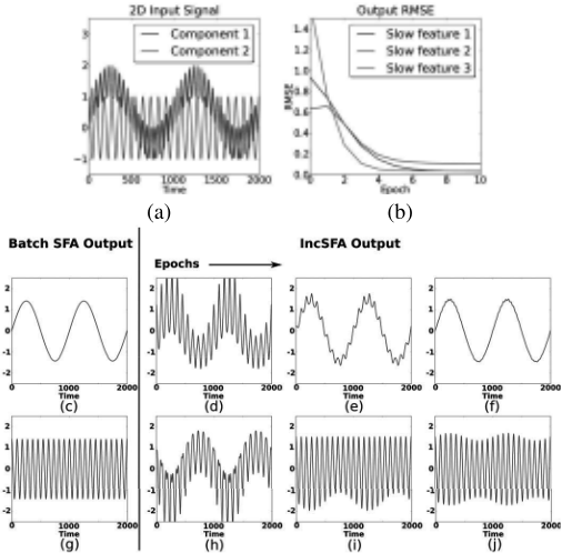
As a basic proof of concept of IncSFA, we tried a problem introduced in the original SFA paper [Wiskott and Sejnowski, 2002]. The input signal is ˘x1(t) = sin(t) + cos(11 t)2 , ˘x2(t) = cos(11 t), t ∈ [0, 2π] - both vary quickly over time (see Figure 1(a)). A total of 2, 000 discrete datapoints are used for learning. The slowest feature hidden in the signal is y1(t) = ˘x1(t) - ˘x2(t)2 = sin(t), and the second is ˘x2(t)2 - these are the features extracted by both batch SFA and IncSFA. Figure 1(b) shows the Root Mean Square Error (RMSE) of output signals compared to the true output, over multiple epochs of training. Figure 1(c) and (g) shows the feature outputs from batch SFA, and (to the right) the IncSFA outputs at 2, 5, and 10 epochs.

6.2 Logistic Map: Complex Signals and High Dimensionality

To test IncSFA's ability to uncover structure hidden in complex signals and high-dimensional data, we use parts of a chaotic time series derived from a logistic map [T. Zito and Berkes, 2008]:

which has a slowly varying driving force γ(t) (to be extracted by IncSFA) hidden in a signal of complicated dynamics. The

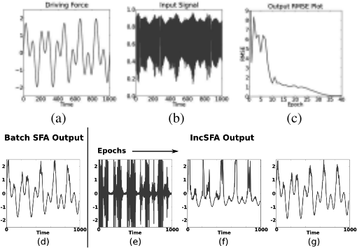
γ(t) used is made up of two frequency components (5 and 11 Hz), given by

Figures 2(a) and 2(b) plot the driving force signal γ(t) and the generated time series ˘x(t), respectively. A total of 1, 000 discrete datapoints are used. To reconstruct the time series, we embed it in a 10 dimensional space using a sliding temporal window of size 10 (we use the TimeFramesNode from the MDP toolkit [T. Zito and Berkes, 2008] for this). The signal is then expanded quadratically to generate an input signal with 65 dimensions. Figure 2(c) shows the convergence of the incremental SFA on the batch SFA output. Figure 2(d) shows the batch SFA output, and Figures 2(e)-(g) show the outputs of the incremental SFA at 15, 30 and 60 epochs.

6.3 2D Exploration: Invariant Spatial Coding

Epochs over the same sequence are not needed; IncSFA also works if data is generated from some movement paradigm which may not lead to exact sequence repetitions.

We use the paradigm of Franzius et al. [Franzius et al., 2007], who fed SFA into ICA to derive computational place cells active at specific agent locations, like those in the rat hippocampus. Such invariant representations of the environment are useful for navigational tasks of organisms or robots.

Our simulated agent performs a random walk in a twodimensional bounded space. Brownian motion is used to generate agent trajectories approximately like those of rats. The agent's position p(t) is updated by a weighted sum of the current velocity and gaussian white noise, with standard deviation vr. The momentum term m can assume values between zero (massless) and one (infinite mass), so that higher values of m lead to smoother trajectories and more homogeneous sampling of space in less time. Once the agent crosses the spatial boundaries, the current velocity is halved and an alternative random velocity update is generated, until a new valid position is reached. Noise variance vr = [3.0, 2.5]T , mass m = 0.75 and 50, 000 data points are used for generating the training set. We use a separate regular grid test dataset for evaluation. Here is the movement paradigm used:

currV el ← p(t) - p(t - 1);

repeat

noise ← GaussianWhiteNoise2d() ∗ vr ;

p(t + 1) ← p(t) + m ∗ currV el + (1 - m) ∗ noise;

if not isInsideWalkArea(p(t + 1)) :

currV el ← currV el/2;

until isInsideWalkArea(p(t +1))

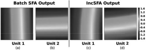
The movement paradigm [Franzius et al., 2007] yields slow feature outputs in the form of half-sinusoids, shown in Figure 3. These features together code for the agent's x and y position in the environment. The first slow feature (Figure 3(a)) is invariant to the agent's x position, the second (Figure 3(b)) to its y position (y axis horizontal). IncSFA's results (Figures 3(c)-(d)) are close to the ones of the batch version, with an RMSE of [0.0536, 0.0914]T .

6.4 High-Dimensional Video: Hierarchical IncSFA

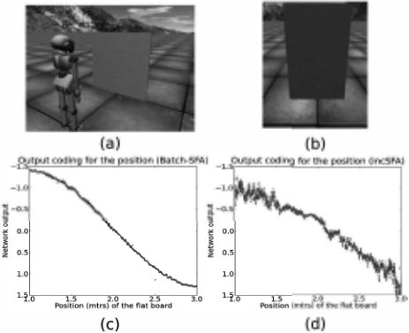
To test the scalability of IncSFA, we feed it with a highdimensional video stream based on 20, 000 images generated by the iCub simulator [V. Tikhanoff and Nori, 2008], an OpenGL-based software specifically built for the iCub robot. Our experiment mimics the robot observing a moving interactor agent, modeled as a rectangular flat board moving back and forth in depth over the range [1, 3] meters in front of the robot, using a movement paradigm similar to the one discussed in Section 6.3. Figure 4(a) shows the experimental setup in the iCub simulator. Figure 4(b) shows a sample image from the dataset. Monocular images were captured from the robot's left eye and downsampled to 83×100 pixels (an input dimension of 8, 300).

Hierarchical Network: We wish the robot to compute features that code for distance. This is a challenging problem, due to the highly nonlinear function mapping pixel intensities to distance. We use a hierarchical model motivated by the human visual system, similar to the one of Franzius et al. [2007].

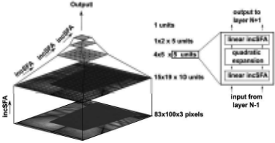
Figure 5 shows the hierarchical architecture, made up of several layers of multiple IncSFA units, acting over overlapping rectangular receptivefields of smaller dimensions. On the lowest layer, the receptive field of each module consists of an image patch of 10 × 10 pixels. The output from the first layer forms a 15 × 19 grid with 10 slow features per each module. With overlapping receptive fields of 5 × 5, this layer's output, with 5 slow features per module, becomes a 4 × 5 × 5 grid. Similarly, third and fourth layers decrease signal dimension to produce one single output. These layers are trained sequentially from bottom to top over the entire dataset.

In general, the number of successfully extracted slow features is only limited by the performance of CCIPCA as compared to batch PCA. Batch PCA can potentially better extract the eigenvectors associated with the smallest eigenvalues as it can iterate over all the data. However, this information, when passed on to our second phase, is rarely useful (for the input data, small eigenvalue directions can typically be removed).

Figures 4 show batch SFA and IncSFA outputs. The expected output is of the form of a sinusoid (refer to Section 6.3) extending over the range of board positions. IncSFA gives a slightly noisy output, probably due to our usage of a constant dimensionality reduction value for all units in each layer of the network, selected to maintain a consistent grid structure. Due to this, some units with eigenvectors having very small eigenvalues emerged in the first stage, with receptive fields observing comparatively few input changes, thus slightly corrupting the whitening result, and adding small fluctuations to the overall result. (Building an adaptive hierarchcial network architecture is one of our future goals.)

A supervised quadratic regressor was trained with ground truth labels on 20% of the dataset, and tested on the other 80%, to measure the quality of features for some classifier or reinforcement learner using them (see RMSE plot). IncSFA derived the driving forces from a complex and continuous input video stream in a completely online and unsupervised manner.

7 Conclusions

IncSFA is the first online algorithm for Slow Feature Analysis, constructed via a combination of incremental PCA and MCA. We showed why IncSFA works and how it resists the curse of dimensionality. IncSFA was successfully compared to batch SFA. To deal with the high nonlinearity involved in extracting slow features from images, a hierarchical IncSFA network was built. It performed well on highdimensional video. IncSFA represents an important step forward, as it opens up the potential of SFA for unsupervised pre-processing of large sets of high-dimensional and/or nonstationary data, such as EEG signals, sensory input streams of autonomous robots, etc.

Acknowledgments

This work was partially funded by the EU project FP7ICT-IP-231722 (IM-CLeVeR) and SNF Sinergia Project CRSIKO-122697.