
Adaptation of a Mixture of Multivariate Bernoulli Distributions
Proceedings of the Twenty-Second International Joint Conference on Artificial Intelligence. Pages 1336-1340.
https://doi.org/10.5591/978-1-57735-516-8/IJCAI11-226
© 2011 International Joint Conferences on Artificial Intelligence
Abstract
The mixture of multivariate Bernoulli distributions (MMB) is a statistical model for high-dimensional binary data in widespread use. Recently, the MMB has been used to model the sequence of packet receptions and losses of wireless links in sensor networks. Given an MMB trained on long data traces recorded from links of a deployed network, one can then use samples from the MMB to test different routing algorithms for as long as desired. However, learning an accurate model for a new link requires collecting from it long traces over periods of hours, a costly process in practice (e.g. limited battery life). We propose an algorithm that can adapt a preexisting MMB trained with extensive data to a new link from which very limited data is available. Our approach constrains the new MMB's parameters through a nonlinear transformation of the existing MMB's parameters. The transformation has a small number of parameters that are estimated using a generalized EM algorithm with an inner loop of BFGS iterations. We demonstrate the efficacy of the approach using the MNIST dataset of handwritten digits, and wireless link data from a sensor network. We show we can learn accurate models from data traces of about 1 minute, about 10 times shorter than needed if training an MMB from scratch.
- [Carreira-Perpiñán and Renals, 2000] Miguel Á. Carreira- Perpiñán and Steve Renals. Practical identifiability of fi- nite mixtures of multivariate Bernoulli distributions. Neu- ral Computation, 12(1):141-152, January 2000.
- [Digalakis et al., 1995] Vassilios V. Digalakis, Dimitry Rtis- chev, and Leonardo G. Neumeyer. Speaker adaptation us- ing constrained estimation of Gaussian mixtures. IEEE Trans. Speech and Audio Process., 3(5):357-366, 1995.
- [Everitt and Hand, 1981] Brian S. Everitt and D. J. Hand. Fi- nite Mixture Distributions. Chapman & Hall, 1981.
- [Gales, 2000] Mark J. F. Gales. Cluster adaptive training of hidden Markov models. IEEE Trans. Speech and Audio Process., 8(4):417-428, July 2000.
- [Gauvain and Lee, 1992] Jean-Luc Gauvain and Chin-Hui Lee. Bayesian learning for hidden Markov model with Gaussian mixture state observation densities. Speech Com- munication, 11(2-3):205-213, June 1992.
- [Gilbert, 1960] E. N. Gilbert. Capacity of a burst-noise chan- nel. Bell Sys. Tech. J., 39(5):1253-1266, September 1960.
- [Kamthe et al., 2009] Ankur Kamthe, Miguel Á. Carreira- Perpiñán, and Alberto E. Cerpa. M&M: Multilevel Markov model for wireless link simulation in sensor net- works. In Proc. of the 7th ACM Conference on Embedded Networked Sensor Systems (SenSys), pages 57-70, 2009.
- [Kuhn et al., 2000] Roland Kuhn, Jean-Claude Junqua, Patrick Nguyen, and Nancy Niedzielski. Rapid speaker adaptation in eigenvoice space. IEEE Trans. Speech and Audio Process., 8(6):695-707, November 2000.
- [Lee and Rose, 1998] Li Lee and Richard Rose. A frequency warping approach to speaker normalization. IEEE Trans. Speech and Audio Process., 6(1):49-60, January 1998.
- [Leggetter and Woodland, 1995] C. J. Leggetter and P. C. Woodland. Maximum likelihood linear regression for speaker adaptation of continuous density hidden Markov models. Computer Speech and Language, 9, 1995.
- [McLachlan and Krishnan, 2008] Geoffrey J. McLachlan and Thriyambakam Krishnan. The EM Algorithm and Ex- tensions. John Wiley & Sons, second edition, 2008.
- [Nocedal and Wright, 2006] Jorge Nocedal and Stephen J. Wright. Numerical Optimization. Springer-Verlag, second edition, 2006.
- [Pawlikowski et al., 2002] Krzysztof Pawlikowski, Hae- Duck Joshua Jeong, and Jong-Suk Ruth Lee. On credibility of simulation studies of telecommunication networks. IEEE Communications Magazine, 40, 2002.
- [Qin and Carreira-Perpiñán, 2009] Chao Qin and Miguel Á. Carreira-Perpiñán. Adaptation of a predictive model of tongue shapes. In Proc. of Interspeech, 2009.
- [Shinoda and Lee, 1997] Koichi Shinoda and Chin-Hui Lee. Structural MAP speaker adaptation using hierarchical pri- ors. In Proc. IEEE Workshop on Automatic Speech Recog- nition and Understanding, pages 381-388, 1997.
- [Thrun and Pratt, 1998] Sebastian Thrun and Lorien Y. Pratt, editors. Learning To Learn. Kluwer, 1998.
- [Woodland, 2001] Phil C. Woodland. Speaker adaptation for continuous density HMMs: A review. In Adaptation Meth- ods for Speech Recognition, ISCA Tutorial and Research Workshop (ITRW), pages 11-19, 2001.
References were extracted automatically from the PDF and may contain errors.
Full text extracted automatically from the PDF; figures, tables and equations may differ. The PDF is the version of record.
1 Introduction
In order to behave optimally, the distributed algorithms running on a sensor network-for example, to find the route for a packet or to decide whether to transmit now or laterrequire knowledge of the wireless link quality between any two nodes. In order to test such algorithms before they run in an actual network, network researchers use simulators that generate binary sequences (data traces) where 1 and 0 correspond to packet reception or loss, respectively. They then generate sequences for as long as desired and feed them to the algorithms as input. Ideally, the distribution of the data traces should match that of the real link targeted. Traditionally, wireless links have been modeled with hand-crafted approaches based on the physics of wave propagation; or with simple statistical models such as the Gilbert-Elliott model [Gilbert, 1960]. However, the former are able to deal only with simple geometries and are unsuitable to real deployments; and the latter may be able to capture simple statistics such as the packet reception rate (PRR, the moving average of the sequence) or simple bursts, but are unable to capture the complex correlations seen in real traces (particularly with low-quality links) [Pawlikowski et al., 2002]. More recently, more sophisticated machine learning methods using larger numbers of parameters estimated on recorded data have shown remarkable improvements. We consider in particular the Multi-level Markov Model (M&M) recently proposed by Kamthe et al. [2009]. This models the binary sequence by considering it as a sequence of windows of W consecutive bits. The model consists of (1) a hidden Markov model (HMM) that accounts for the long-term changes in the sequence, mostly caused by drastic changes in the PRR (e.g. caused by interference by an object moving nearby); and (2) as output distribution of each HMM state, a mixture of multivariate Bernoulli distributions (MMB) that accounts for short-term changes intrinsic to the link (dependent on its location). Kamthe et al. trained this model on long data traces (over hours or days) and showed using various statistics (PRR, run length distribution, Jensen-Shannon divergence) the ability of the M&M model to learn complex distributions for links of very different characteristics.
However, one drawback of the M&M and similar datadriven models with many parameters is the need for sufficiently large training sets to achieve reliable estimates. This means that for each link of a sensor network that we want to model, the network developer must first record data for enough time (hours or days). This prevents quick setup of a new link and is costly in resources (e.g. battery life), particularly for sensors in hard-to-reach locations (such as climatesensing networks in Greenland). In these situations, it makes sense to use an existing model (which we call reference) that has been trained with extensive data and adapt it to the new situation (the target distribution) given a far smaller data trace than would be necessary to train a new model from scratch. This is the adaptation setting that we pursue in this paper.
In the original M&Mmodel [Kamthe et al., 2009], one first clusters the training set into separate subsets roughly corresponding to different PRRs, and each cluster corresponding to one state of the HMM. Then a different MMB is learned separately for each state. Thus, we focus here on adapting not the entire M&M model but on adapting a single MMB. We assume that the data corresponding to this particular MMB has been selected ahead of time. We believe ours is the first approach to adapting a mixture of multivariate Bernoullis.
In the next sections, we review related work, define the MMB and our adaptation strategy, derive a generalized EM algorithm, and evaluate it with MNIST and wireless data.
Related work In machine learning, work on transfer and multitask learning has considered the problem of learning models such as classifiers in the presence of different domains [Thrun and Pratt, 1998]. In our adaptation setting, we do not know at training time the target distribution we need to model. Our work is most closely related to adaptation methods in speech processing [Woodland, 2001], where given a Gaussian-mixture-based HMM trained for a reference speaker we want to adapt it to a new speaker given as little new speech as possible. Maximum-a-posteriori methods apply Bayes' rule using as prior the trained model [Gauvain and Lee, 1992] or a hierarchical prior [Shinoda and Lee, 1997] and converge to the true maximum-likelihood estimate with infinite data, but are generally not competitive with little adaptation data because only a few parameters are updated. Thus, most work is based on tying together groups of parameters (means, covariances) and using linear transformations of the parameters or features [Leggetter and Woodland, 1995; Digalakis et al., 1995; Lee and Rose, 1998; Qin and CarreiraPerpi˜n´an, 2009]. This does not converge to the maximumlikelihood estimate but updates all parameters and significantly improves the model with little data. As we show later, linear transformations are not suitable with MMBs because (unlike the means of a Gaussian) the prototypes are constrained to be in [0, 1].
Other work considers a space where each point represents a model, and constrains the target model to be in a manifold or cluster set spanned by existing trained models [Kuhn et al., 2000; Gales, 2000]. However, this requires sufficiently many trained models, which may not be available in practice.
2 Mixture of multivariate Bernoulli distributions
Beyond its use in the M&M model, mixtures of multivariate Bernoulli distributions (MMB) are widely used to model high-dimensional binary data in terms of a few latent classes, from bacterial taxonomy to binary images [Everitt and Hand, 1981; Carreira-Perpi ˜n´an and Renals, 2000]. Given a data vector x ∈ {0, 1}W with W binary variables, its density is
where there are M components and the parameters are the mixing proportions πm (which are positive and sum to one) and the prototypes pm ∈ [0, 1]W . Thus, variables within a component are independent, but not across components. With enough components, an MMB can represent complex highdimensional distributions.
Given a training set, an MMB is usually trained with an EM algorithm. The E step computes the posterior probability of each component given a data vector. The M step estimates the parameters of each component: its mixing proportion is proportional to the total posterior probability of the component, and its prototype is the average of the whole data wrt the posterior probabilities. The EM algorithm needs initial values for the parameters and can converge to local optima.
In the context of adaptation, we will call retraining the process of estimating an MMB using this EM algorithm given the adaptation data, and initializing the parameters to those of the reference MMB. Retraining with little data leads to estimates that overtrain and generalize poorly to future data. For example, in applications like those we consider (binary images or windows), the space dimensionalityW is large (hundreds), so if little adaptation data is available, some of the dimensions in the data may consist mostly (or only) of 0s or 1s. The correspoding pmw value will clamp to (close to) 0 or 1 and will then rarely generate a 1 or a 0, respectively, during sampling, so the simulated traces will not be representative of the data.
3 Adapting the MMB
We now assume we have an MMB model (the reference model) that has been trained on an extensive dataset (say, from a given wireless link in a network), that is, we have the values of its parameters (mixing proportions and prototypes). We are given an adaptation dataset, sampled from an unknown target distribution, containing a small number N of binary W-dimensional vectors {xn}Nn=1, and we want to learn a new MMB model, with parameters {˜ πm, ˜pm}Mm=1, for the target distribution. Our algorithm is based on the idea of tying the MMB parameters together through a transformation of the reference parameters. The transformation itself has very few parameters, so they can be learned from the small adaptation dataset, but their effect is propagated to all the MMB parameters through the transformation. Specifically, we obtain each new W-dimensional prototype ˜ pm as a nonlinear transformation f (pm, θm) of the reference prototype pm, independently for each component, using a number of parameters θm much less than W. The transformation is nonlinear because the prototypes must be in [0, 1]. With a linear transformation with shared parameters, the total amount of change in pm is limited, because reference values pmw close to either 0 or 1 would immediately reach 0 or 1 (saturate) and prevent the remaining, less extreme values from adapting. This is a major difference with existing adaptation work on Gaussian mixtures where the Gaussian means are unconstrained and linear transformations suffice. In this paper, we apply a sigmoid transformation with parameters am, bm ∈ R elementwise to each entry in pm:
This allows large changes to all pmw even if some are close to the boundaries. (In the nongeneric case where all pmw values are identical within one component, there is an infinite number of (am, bm) values that can map it to a given output, and our algorithm will find one of those.) As for the mixing proportions, since there is only one per component, we consider them as free during adaptation (subject to adding to 1).
Thus, our algorithm needs to maximize the likelihood of the adaptation data over a total of 3M - 1 free parameters (mixing proportions ˜ π1, . . . , ˜ πM-1 and sigmoid parameters a1, b1, . . . , aM, bM), which with our high-dimensional data is far less than (W + 1)M - 1 parameters (proportions and prototypes) for the unconstrainedMMB.
Like the EM algorithm for MMBs, our GEM algorithm can converge to local optima. Since the point of adaptation is that the reference model should be relatively close to the target one, the initial values for {˜ πm, am, bm} should be such that the MMB they represent is as close as possible to that of the reference model. This is achieved by setting ˜ πm = πm and am = 5.47, bm = -2.79; the latter correspond to the sigmoid that is closest to the identity transformation. We do describe an alternative initialization strategy in section 5.
A generalized EM algorithm for adaptation Our objective function is the log-likelihood of the adaptation data given the constrained MMB model with 3M - 1 free parameters:
L ({˜ πm, am, bm}Mm=1) = ∑Nn=1 log ∑Mm=1 ˜ πmp(xn; am, bm) where p(xn; am, bm) is a multivariate Bernoulli with prototype ˜pm = σ(pm; am, bm). We provide a generalized expectation-maximization (EM) to maximize it [McLachlan and Krishnan, 2008]. Unlike in the EM algorithm to train an MMB, the use of a nonlinear transformation makes the M step now not solvable in closed form for {am, bm}. Instead, we need to solve it iteratively; we have found the BFGS algorithm (a quasi-Newton algorithm with superlinear convergence; Nocedal and Wright [2006]) effective. Since this increases but (if we exit BFGS early) need not maximize the likelihood within the M step, our EM algorithm is generalized, and the theorems for convergence of GEM apply [McLachlan and Krishnan, 2008]. The E step is analogous to that of the EM algorithm for MMBs. In the equations below, note ˜ pτmw = σ(pmw; aτm, bτm).
- E step This computes rτmn = p(m|xn; ˜ πτm, aτm, bτm), the posterior probability of component m given data point xn under the current iteration's (τ) parameters:
M step This results from increasing or maximizing Q, the expected (wrt the rτmn) complete-data log-likelihood, over ˜ πm, am, bm:
∑Nn=1 ∑Mzn=1 rτ zn,n log (p(zn; ˜ πzn )p(xn|zn; azn , bzn )) where we call 1 ≤ zn ≤ M the (unknown) index of the mixture component that generated data point xn. We obtain a closed-form solution for the mixing proportions:
but the expression for the gradient of Q wrt {am, bm}
when equated to zero cannot solved in closed form for {aτ +1 m , bτ+1 m }, so we iterate over {am, bm} using BFGS.
Computational complexity Our algorithm consists of an outer loop of GEM iterations, and an inner loop of BFGS iterations for the M step. Our experiments show how to set the exit tolerance and maximum number of inner-loop iterations. Computing the BFGS search direction is O(M 2 ) (a matrix-vector product of order M), which is negligible wrt computing the E step and gradient of Q, both of which cost O(MNW). Thus the algorithm runtime is O(NMW) times the total number of inner-loop iterations.
4 Experiments
4.1 MNIST handwritten digits
The MNIST dataset, commonly used in machine learning, contains grayscale images of 28 × 28 pixels (W = 784 dimensions) of handwritten digits from many writers. We illustrate our adaptation algorithm by having a reference model trained on a large subset of MNIST, and then adapting to a small subset where the pixel intensities have been inverted (see fig. 1). This represents a situation where the target distribution is very different from the reference distribution, but many of its characteristics (e.g. digit class, slant, thickness) do not change. These characteristics have been learnt by the reference model using a large training set, and the goal of the adaptation is to preserve those but change the intensity to match the new, inverted one.
We used data from the digits '1', '2' and '3' only. We randomly split the 10000 digits per class into a training set (3 000), a target dataset (6 000) and a test dataset (1 000). Although MNIST provides the digit label, none of our experiments use it, so all models are learnt in a purely unsupervised way. We converted the grayscales from [0, 1] to binary using a threshold of 0.5, and inverted the images from the target and test sets. Our reference model (fig. 2) had M = 3 components (for a total of 2 354 parameters) and was learned on the training set with the EM algorithm. For adaptation (8 parameters) and retraining (2354 parameters), we used randomly selected subsets of size N from the target set, where N varied from 3 to 18 000 (the whole target set); note that subsets did not necessarily contain the same number of '1', '2' or '3'. The experiments were repeated over 50 subsets each to obtain errorbars. As initialization, we used the algorithm described in section 5 for both EM retraining and GEM adaptation. We stopped iterating when the relative log-likelihood change was less than 10-8.
Fig. 2 shows the learned parameters for a particular subset of N = 100 adaptation vectors. The parameters resulting from adaptation resemble very much the ones resulting from retraining with extensive data, which in turn resemble the reference ones but inverted (also shown by the inverted sigmoids in fig. 3). The prototypes look like smooth, average shapes representative of the entire populations of '1', '2' and '3'. Even though we adapt only 8 free parameters, all 2 354 parameters (prototypes and proportions) undergo large changes. However, retraining with N = 100 vectors gives poor results, with each component learning slant and other traits that are idiosyncratic to the particular adaptation set used.


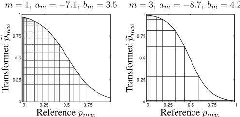
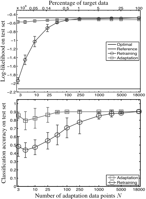
Fig. 4(top) shows the log-likelihood on the test set as a function of N. The adaptation algorithm achieves results close to retraining with all data ("optimal" line) for very small N and reliably so (note the tight errorbars). As N increases, the adaptation performance stagnates without reaching the optimal baseline, a necessary consequence of learning very few free parameters. Retraining needs N > 100 vectors to equal adaptation and performs poorly and unreliably with small N. The classification accuracy (fig. 4, bottom), where we assigned a test image x to the cluster with largest posterior probability p(m|x) under the MMB, shows similar results.
We also determined the number of inner-loop iterations (which correlates well with the runtime) that leads to fastest runtime. We ran the inner loop until either a relative loglikelihood change of ϵ or I iterations were achieved, for a fixed model initialized from the same point (we checked all repeats converged to the same optimum). Table 1 shows that solving the inner, BFGS iteration accurately is fastest, and we used ϵ = 10-8 and I = 25 for all our experiments.
| Fixed I | Fixed ϵ | ||||||
|---|---|---|---|---|---|---|---|
| ϵ | I | outer | inner | ϵ | I | outer | inner |
| 10-1 | 100 | 267 | 267 | 10-8 | 1 | 267 | 267 |
| 10-2 | 100 | 281 | 284 | 10-8 | 2 | 27 | 53 |
| 10-3 | 100 | 343 | 365 | 10-8 | 3 | 34 | 96 |
| 10-4 | 100 | 157 | 171 | 10-8 | 4 | 30 | 117 |
| 10-5 | 100 | 47 | 62 | 10-8 | 5 | 26 | 126 |
| 10-6 | 100 | 3 | 20 | 10-8 | 10 | 4 | 23 |
| 10-7 | 100 | 3 | 20 | 10-8 | 25 | 3 | 20 |
| 10-8 | 100 | 3 | 20 | 10-8 | 100 | 3 | 20 |
4.2 Wireless link data
We collected a comprehensive database of packet reception traces of links having different reception rates using 802.15.4 compliant CC2420 radios. The nodes were deployed indoors along the ceiling of a corridor in an office building. In our experiments, we have one fixed sender and multiple receivers. The sender sends 64 packets per second with an interpacket interval of 16 ms for 1 hour, so the length of each packet reception trace is 230 400 bits for each link. We treat one of the links as the reference link and all other links as target links; for the latter, each 1-hour trace is split 70/30 into target and test data.
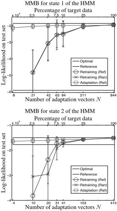
Using the trace for the reference link, we estimated a reference M&M model as described by Kamthe et al. [2009] using a 2-state HMM (so we have one MMB for each), M = 5 components per MMB and a window of W = 128 bits. The experimental setup then proceeded as with the MNIST data, except we initialized the models from the reference (retraining) or the identity transformation (adaptation), and we assigned target and test data to states according to their packet reception rate (PRR). We then retrained/adapted each MMB over target datasets of size N and reported the log-likelihood (fig. 5) on the tests traces, all collected from a link different from the reference. Again, we see that adaptation needs far less data (about 10 times less), although stagnation does occur for larger adaptation set sizes. Using a total of around N = 30 vectors (20 and 10 for states 1 and 2, respectively) achieves a log-likelihood very close to that retraining on the entire target data. At a rate of 64 packets/s, this means 1 minute recording time.
We also embedded the adapted or retrained MMBs in the M&M model and generated long traces from it on different links. Statistics from these (data not shown), such as run length distributions, again confirm that adaptation needs about 10 times less data than retraining. Given the limits on battery life of sensors, this makes a crucial difference.
5 Discussion
In a parameter-sharing adaptation approach, the goal is to learn a few transformation parameters from the scarce adaptation data such that they can propagate the new information to all the MMB parameters. Our choice of transformation and parameter-sharing is driven by two facts: the data dimensionality W is large and quite larger than the number of components M; and in a wireless link, we suspect that changes in the distribution are often caused by across-the-board changes in the packet reception rate, which push up or down all the prototype entries. Thus, having two parameters am, bm per component that apply elementwise makes sense, and our experiments confirm this. However, this is not the only sharing strategy, nor do we expect it to perform well in all circumstances. For example, sharing across dimensions rather than components, adding a new component with W entirely free parameters, or sharing parameters in a more complex way, might be suitable to other settings.
It is interesting to see the (re)training EM algorithm and our adaptation GEM algorithm from the perspective of clustering, assignments and fitting. If we had a single component, the retraining and adaptation to a dataset would be a trivial fit: retraining would set p1 to the mean of the data, and adaptation would fit a sigmoid σ(p; a1, b1) that best maps (elementwise) the reference p1 to the data mean. With several components (M > 1), the retraining needs to solve a clustering problem (which of the N data points xn go to which of the M clusters) and a fitting problem (of each prototype to the mean of its cluster). The MMB EM algorithm solves this (in a soft way, using posterior probabilities of components corresponding to data points), and can have local optima; which one we find depends on the initial {πm, pm}Mm=1. With several components, the adaptation needs to solve a clustering problem (as before), an assignment problem (which component of the reference MMB goes to which cluster of the data) and a fitting problem (as before). Again, our GEM adaptation algorithm solves this in a soft way, and can have local optima depending on the initial {˜ πm, am, bm}Mm=1 . This also suggests a simple, suboptimal algorithm to estimate the parameters, where these three problems are solved sequentially:
- Clustering: cluster the data intoM clusters with k-means.
- Assignment: assign reference prototypes to nearestneighbor k-means centroids in a one-to-one correspondence (e.g. by selecting neighbors greedily).
- Fitting: for each component separately, find the best sigmoid that maps the reference prototype to the centroid.
The resulting {am, bm} or {pm} will likely be suboptimal, particularly with sparse adaptation data, but can be used as an alternative initialization for the EM and GEM algorithms.
6 Conclusion
We have proposed what, as far as we know, is the first approach to quickly adapt a reference MMB model to a new distribution given a few samples from the latter. We nonlinearly and separately transform each prototype from the reference MMB using a small number of parameters and estimate these with a generalized EM algorithm. In our current sensor network infrastructure, this achieves models with traces of about a minute that are about as good as retraining all MMB parameters from scratch with traces of hours, greatly simplifying the task of building realistic network simulators. Our algorithm applies to adapting MMBs in other settings, although we expect that other ways of sharing parameters may be more suitable, and future work should address this.
Matlab code available at http://eecs.ucmerced.edu.
Acknowledgments
Work partially supported by the National Science Foundation under grants IIS-0711186 and CNS-0923586, the California Institute for Energy and Environment under grant MUC-0903, and the Center for Information Technology Research in the Interest of Society under grant 442130-19900.
@inproceedings{ijcai2011p226,
  title     = {Adaptation of a Mixture of Multivariate Bernoulli Distributions},
  author    = {Kamthe, Ankur and Carreira-Perpiñán, Miguel Á. and Cerpa, Alberto},
  booktitle = {Proceedings of the Twenty-Second International Joint Conference on
               Artificial Intelligence, {IJCAI-11}},
  publisher = {AAAI Press/International Joint Conferences on Artificial Intelligence},
  editor    = {Toby Walsh},
  pages     = {1336--1340},
  year      = {2011},
  month     = {7},
  doi       = {10.5591/978-1-57735-516-8/IJCAI11-226},
  url       = {https://doi.org/10.5591/978-1-57735-516-8/IJCAI11-226},
}
TY - CPAPER TI - Adaptation of a Mixture of Multivariate Bernoulli Distributions AU - Kamthe, Ankur AU - Carreira-Perpiñán, Miguel Á. AU - Cerpa, Alberto T2 - Proceedings of the Twenty-Second International Joint Conference on Artificial Intelligence, IJCAI-11 PB - AAAI Press/International Joint Conferences on Artificial Intelligence PY - 2011 SP - 1336 EP - 1340 DO - 10.5591/978-1-57735-516-8/IJCAI11-226 UR - https://doi.org/10.5591/978-1-57735-516-8/IJCAI11-226 ER -Copied
Machine-readable versions of this paper, for tools and AI agents:





