
Feature Selection via Joint Embedding Learning and Sparse Regression
Proceedings of the Twenty-Second International Joint Conference on Artificial Intelligence. Pages 1324-1328.
https://doi.org/10.5591/978-1-57735-516-8/IJCAI11-224
© 2011 International Joint Conferences on Artificial Intelligence
Abstract
The problem of feature selection has aroused considerable research interests in the past few years. Traditional learning based feature selection methods separate embedding learning and feature ranking. In this paper, we introduce a novel unsupervised feature selection approach via Joint Embedding Learning and Sparse Regression (JELSR). Instead of simply employing the graph laplacian for embedding learning and then regression, we use the weight via locally linear approximation to construct graph and unify embedding learning and sparse regression to perform feature selection. By adding the l2,1-norm regularization, we can learn a sparse matrix for feature ranking. We also provide an effective method to solve the proposed problem. Compared with traditional unsupervised feature selection methods, our approach could integrate the merits of embedding learning and sparse regression simultaneously. Plenty of experimental results are provided to show the validity.
- [Belkin and Niyogi, 2003] Mikhail Belkin and Partha Niyogi. Laplacian eigenmaps for dimensionality reduction and data rep- resentation. Neural Comput., 15:1373-1396, 2003.
- [Cai et al., 2007] Deng Cai, Xiaofei He, and Jiawei Han. Spectral regression for efficient regularized subspace learning. In Proc. Int. Conf. Computer Vision (ICCV'07), 2007.
- [Cai et al., 2010] Deng Cai, Chiyuan Zhang, and Xiaofei He. Unsu- pervised feature selection for multi-cluster data. KDD '10, pages 333-342, 2010.
- [Dash et al., 2002] Manoranjan Dash, Kiseok Choi, Peter Scheuer- mann, and Huan Liu. Feature selection for clustering -a filter solution. ICDM '02, pages 115-122, 2002.
- [Dy et al., 2004] Jennifer G. Dy, Carla E. Brodley, and Stefan Wro- bel. Feature selection for unsupervised learning. Journal of Ma- chine Learning Research, 5:845-889, 2004.
- [He et al., 2005] Xiaofei He, Deng Cai, and Partha Niyogi. Lapla- cian score for feature selection. In NIPS, 2005.
- [Krzanowski, 1987] W. J. Krzanowski. Selection of Variables to Preserve Multivariate Data Structure, Using Principal Compo- nents. Journal of the Royal Statistical Society. Series C (Applied Statistics), 36(1):22-33, 1987.
- [Nie et al., 2008] Feiping Nie, Shiming Xiang, Yangqing Jia, Changshui Zhang, and Shuicheng Yan. Trace ratio criterion for feature selection. In AAAI, 2008.
- [Nie et al., 2010a] Feiping Nie, Heng Huang, Xiao Cai, and Chris Ding. Efficient and robust feature selection via joint l 2,1-norms minimization. In NIPS 23. 2010.
- [Nie et al., 2010b] Feiping Nie, Dong Xu, Ivor Wai-Hung Tsang, and Changshui Zhang. Flexible manifold embedding: A frame- work for semi-supervised and unsupervised dimension reduction. IEEE TIP, 19(7):1921-1932, 2010.
- [Roth and Lange, 2004] Volker Roth and Tilman Lange. Feature selection in clustering problems. In NIPS 16, 2004.
- [Roweis and Saul, 2000] Sam T. Roweis and Lawrence K. Saul. Nonlinear dimensionality reduction by locally linear embedding. Science, 290:2323-2326, 2000.
- [Zhao and Liu, 2007] Zheng Zhao and Huan Liu. Spectral feature selection for supervised and unsupervised learning. In ICML, pages 1151-1157, 2007.
- [Zhao et al., 2010] Zheng Zhao, Lei Wang, and Huan Liu. Efficient spectral feature selection with minimum redundancy. In AAAI, 2010.
References were extracted automatically from the PDF and may contain errors.
Full text extracted automatically from the PDF; figures, tables and equations may differ. The PDF is the version of record.
1 Introduction
The problem of reducing data's dimensionality is a key research topic for both artificial intelligence and machine learning. In the literature, there are mainly two distinct ways for dimensionality reduction: feature selection and feature learning (or 'feature extraction'). Feature selection tries to extract a few relevant features to represent the original data while feature learning combines several original features to form new representations. Compared with feature learning which can create new features, feature selection does not change the original representations of data variables. If we are required to keep the original physical meanings of each feature, feature selection is preferred. Additionally, there is another advantage for feature selection. When we have determined the selected features, we only need to calculate or collect these concerning features. In feature learning, however, all features are still needed for dimensionality reduction.
Consequently, many researches have been proposed to address the problem of feature selection in the past few years. There are mainly two different kinds of feature selection approaches: supervised and unsupervised. Since we have no label information in unsupervised feature selection, it is more difficult than supervised scenario and there are relatively fewer investigations dedicated to this topic. Most unsupervised feature selection approaches are either based on filters [Dash et al., 2002] [Nie et al., 2008], wrappers [Roth and Lange, 2004] or embeddings [Dy et al., 2004]. Although the performances of traditional unsupervised feature selection approaches are prominent in many cases, their efficiencies can also be improved since (1) from the view of manifold learning [Cai et al., 2007], the high dimensional data are nearly lying on a low dimensional manifold. Traditional methods have not taken fully considerations about the manifold structure. (2) Different from feature learning, traditional feature selection approaches only employ data statistical character to rank the features essentially. They are often lack of using the learning mechanism as in feature learning, which is proved to be powerful and widely used in many areas [Nie et al., 2010b].
Recently, to leverage both the manifold structure and learning mechanism, some investigations have emerged. Typical methods include: Pca Score (PcaScor) [Krzanowski, 1987], Laplacian Score (LapScor) [He et al., 2005], Spectral Feature Selection (SPEC) [Zhao and Liu, 2007], Multi-Cluster Feature Selection (MCFS) [Cai et al., 2010] and Minimum Redundancy Spectral Feature selection (MRSF) [Zhao et al., 2010]. Commonly, these methods use various graphs to characterize manifold structure at first. LapScor and SPEC then compute different metrics to rank each feature. MCFS and MRSF, however, add sparse constraints in multi-output regression. Compared with traditional unsupervised feature selection approaches, these methods have proved to perform better in many cases [Zhao et al., 2010]. Nevertheless, their performances can also be improved since these methods all separate manifold characterization and feature selection. Once the graph is determined to characterize manifold structure, it is fixed in the following ranking or regression steps. Thus, the performance of feature selection is largely determined by the effectiveness of graph construction. On the contrary, if the graph laplacian can adaptively change w.r.t. the following ranking or regression procedures, i.e., the graph not only can characterize manifold structure, but also indicate the requirements of regression, these methods would perform better.
In this paper, we introduce a novel unsupervised feature selection approach via Joint Embedding Learning and Sparse Regression (JELSR). Instead of simply using the graph laplacian to characterize high dimensional data's structure and then regression, we propose to adopt locally linear approximation weight to construct a new graph and unify these two objectives in forming a new problem. By adding the ℓ2,1norm regularization, we can learn a sparse transformation matrix for feature selection. We also provide an effective method to solve the proposed problem. Compared with traditional unsupervised feature selection approaches, our method could integrate the merits of manifold learning and sparse regression. Many experimental results are provided for demonstration.
The rest of this paper is organized as follows. We will formulate JELSR and provide an effective solution algorithm in Section 2. Section 3 will present the convergence behavior and relations to other approaches. Section 4 provides some comparing results on various kinds of data sets, followed by the conclusion and future works in Section 5.
2 Feature Selection via Joint Embedding Learning and Sparse Regression
In this section, we will first introduce some notations. The concrete formulation is then proposed. Finally, we provide an effective algorithm to solve this problem.
Before going into the details of our algorithm, let us introduce some notations. Denote {xi ∈ Rd |i = 1, 2, · · · , n} as the unlabeled examples. We would like to select s features to represent the original data, where s < d. For a matrix Q ∈ Ru×v , its ℓr,p-norm is defined as follows.
For brief, the ℓ2-norm is also denoted as ‖ · ‖2 in the following. Define α > 0, β > 0 as two balance parameters.
2.1 Formulations
There are mainly three objective functions of our algorithm. We would like to introduce them in sequence.
Considering that Spectral Regression (SR) performs well in feature learning and graph laplacian could fully characterize manifold structure, we would like to inherit their advantages in formulating our feature selection algorithm. Evoked by the intuition that nearby points should have similar properties, we would like to construct a weight graph G = (V, E, S) to reveal their local connections, where V = {xi} is the graph vertex set and E contains edges of the constructed graph.
The key point in constructing graph is to determine its weight matrix S, where Sij reveals the similarity between points xi and xj . Commonly, the graph is constructed by connecting every point to its k-nearest neighbors and the weights for connected points are computed by gaussian function. Motivated by the prominent performance in using locally linear approximation weight to construct graph [Roweis and Saul, 2000], we would like to employ similar strategy to measure local similarity. More concretely, the graph is constructed by following steps:
Step 1. Constructing a k-nearest graph G. The i-th node corresponds to xi. For xi, it only connects with the points in its k-nearest neighborhood set N(xi). Thus, G is a directed graph.
Step 2. Computing the similarity matrix S. For the i-th point xi, its weight Sij > 0 if and only if xj ∈ N(xi). Otherwise, Sij = 0. The nonzero weight is determined by using the following locally linear approximation strategy.
Recalling the basic idea of feature learning, we will represent the original data xi by its low dimensional embedding, i.e., yi ∈ Rm, where m is the dimensionality of embedding. Through this kind of replacement, the most valuable information is retained and the feature redundancies are eliminated. As a result, the first objective is
where L = (In×n - S)T (In×n - S) is the graph laplacian. yi ∈ Rm is the embedding of xi for i = 1, 2, · · · , n and Y = [y1, y2, · · · , yn].
As in SR, the second objective function of our algorithm is to regress each sample to its low dimensional embedding. More concretely, assume {xi} is centered and denote W = [w1,w2, · · · ,wm] ∈ Rd×m as the matrix formulated by all transformation vectors {wi}mi=1 , the second objective function is
The third objective function is designed for feature selection. Denote ˆwi as the i th row vector ofW, i.e.,
Essentially, ˆwi corresponds to the transformation vector of the i-th feature in regression. It can also be regarded as a vector that measures the importance of the i-th feature.
Considering the task of feature selection, we expect that the transformation matrix holds the sparsity property for feature selection. More concretely, we expect that only a few numbers of ˆwi are non-zeros. As a result, the corresponding features are selected since these features are enough to regress the original data xi to its low dimensional representation yi. When we employ the 2-norm of ˆwi as a metric to measure its contribution in this regression, the sparsity property, i.e., a small number of ˆwi are non-zeros, indicates the following objective function.
Here ‖W‖2,1 denotes the ℓ2,1-norm as defined in Eq. (1).
By combining the objective functions in Eq. (3), Eq. (4) with Eq. (6), our JELSR algorithm can be formulated as follows.
where α and β are two balance parameters.
After deriving W, we use the 2-norm of ˆwi, i.e., ‖ˆwi‖2 to rank the features. The larger ‖ˆwi‖2 is, the more important this feature is. We can either select a fixed number of the most important features or set a threshold and select the feature whose ‖ˆwi‖2 is larger than this value. In the following, we select a fixed number, i.e., s, features for evaluation.
2.2 Solutions
Considering the optimization problem in Eq. (7), since we have added the ℓ2,1-norm regularization for feature selection, it is hard to derive its closed solution directly. Inspired by [Nie et al., 2010a], we will solve this problem in an alternative way. As we will explain later, through this kind of procedure, we update the embedding Y and the sparse regression matrixWalternatively. In other words, we select the features by joining embedding learning and sparse regression, which has not been considered in the literature.
Note that ‖W‖2,1 is convex. Nevertheless, its derivative does not exist when ˆwi = 0 for i = 1, 2, · · · , d. For convenience, we would like to denote L(W) = ‖WT X-Y‖22 + α‖W‖2,1. Thus, when ˆwi ̸= 0 for i = 1, 2, · · · , d, the derivative of L(W) w.r.t. W is
where U ∈ Rd×d is a diagonal matrix whose i-th diagonal element is
As seen from Eq. (8), we construct an auxiliary function. It is obvious that the derivative in Eq. (8) can also be regarded as the derivative of the following objective function.
Consequently, we try to solve the following problem to approximate the solution to Eq. (7).
where U is defined as in Eq. (9).
We would like to explain why we can deriving a sparse solution by minimizing Eq. (11). Recalling the definition of Uii in Eq (9), we know that tr(WT UW) = ‖W‖2,1/2 when ˆwi is not equal to 0. Thus, the objective of minimizing tr(WT UW) will add the sparsity constraint on W. Intuitively, if ‖ˆwi‖2 is small, then Uii is large and the minimization of Eq. (10) tends to derive ˆwi with much smaller ℓ2norm. After several times of iteration, the norms of some ˆwis are close to zero and we get a sparseW. Besides, the above approximation can not be used if ˆwi ̸= 0 for i = 1, 2, · · · , d.
As seen from above formulation, the objective function in Eq. (11) is convex with respect to W and Y if U is fixed. When W is fixed, we can determine U by Eq. (9) directly. Thus, we update W and Y when U is fixed and compute U when W is fixed.
When U is fixed, we would like to take the derivative of L(W,U,Y) with respect to W and set it to zero, i.e., we have the following equation.
or equivalently,W = (XXT
By substituting above W into Eq. (11), we will have
Considering the objective function in Eq. (15) and the constraint YYT = Im×m, the optimization problem becomes
If A and L are fixed, the optimization problem in Eq. (16) can be solved by eigen-decomposition of matrix (L + βIn×n - βXT A-1X). We pick up the eigenvectors corresponding to the m smallest eigenvalues.
When W is fixed, we can update U by employing the formulation in Eq. (9) directly.
In summary, we solve the optimization problem in Eq. (7) in an alternative way. More concretely, if U is fixed, we can first solve the optimization problem in Eq. (16) to update Y and then employ Eq. (13) to updateW. After that, we fixW and update U, which is defined in Eq. (9).
We now explain why our method could join embedding learning and sparse regression. Considering the above algorithm, we solve the problem in Eq. (16) to compute Y. In other words, the objective of sparse regression has also affected the derivation of low dimensional embedding, i.e., Y. Traditional methods, such as MCFS and MRSF, minimize tr(YLYT ) merely.
Additionally, since JELSR is solved in an alternative way, we would like to initialize U by an identity matrix. The experimental results show that our algorithm converges fast by using this kind of initialization. The number of iteration is often less than twenty. Besides, the above solving procedure can not be used when ˆwi = 0 for i = 1, 2, · · · , d. This is another reason why we use this type of initialization.
In summary, the procedure of JELSR is listed in Table 1.
Table 1: Procedure of JELSR.
Input: Data set {xi|i = 1, 2, · · · , n}; Balance parameter α β; Neighborhood size k; Dimensionality of embedding m; Selected feature number s.
Output: Selected feature index set {r1, r2, · · · , rs}.
Stage one: Graph construction
- Construct the nearest neighborhood graph G;
- Compute the similarity matrix S, graph laplacian L;
Stage two: Alternative optimization
- Initialize U= Id×d;
- Alternatively update U, Y and W until convergence.
- Fix U, update Y by solving the problem in Eq. (16), updateWby using Eq. (13);
b. FixW, update U by Eq. (9);
Stage three: Feature selection
- Compute the scores for all features {‖ ˆwi‖2}di=1 ;
- Sort these scores and select the largest s values. Their corresponding indexes form the selected feature index set {r1, r2, · · · , rs}.
3 Discussions
In this section, we will analyze JELSR in two aspects, i.e., the convergence behavior and the relations to other approaches.
3.1 Convergence Analysis
As seen from Table 1, since we have solved JELSR in an alternative way, we would like to show its convergence behavior. First, a lemma [Nie et al., 2010a] is provided.
Lemma 1. For any non-zero vectors a, b ∈ Rm, the following result follows
The convergence behavior of JELSR is summarized in the following theorem.
Theorem 1. The optimization procedure in the second stage of Table 1 will monotonically decrease the objective of the problem in Eq. (7) in each iteration.
Proof. As seen from the algorithm in Table 1, when we fix U as Ut in the t-th iteration and compute Wt+1 , Yt+1 , the following inequality holds,
Since ‖W‖2,1 = ∑di=1 ‖ˆwi‖2, the above inequality indicates
Recalling the results in Lemma 1, we know that
Combining Eq. (19) with Eq. (20), we have the following results.
This inequality indicates that the objective function in Eq. (7) will monotonically decrease in each iteration.
Additionally, since the objective function has lower bounds, such as zero, the above iteration will converge. Besides, the following experimental results show that it converges fast, the time of iteration is often less than 20.
3.2 Relations to other Approaches
First, considering the above deduction of our algorithm, we know that JELSR is related to LapScor [He et al., 2005]. LapScor selects features that can best preserve the similarity revealed by S. Both JELSR and LapScor construct a graph to characterize data manifold. JELSR uses the locally linear approximation weights while LapScor employs the gaussian function. Compared with LapScor, JELSR uses a more prominent way, i.e., sparse regression, to learn feature weights. It could inherit the metric of SR [Cai et al., 2007]. Moreover, SPEC is also based on spectral analysis and it can be regarded as an extension of LapScor. Nevertheless, SPEC exploits both labeled and unlabeled data through a regularization framework and emphasizes the problem of semi-supervised feature selection. JELSR, however, focuses on the unsupervised case.
Second, JELSR has close relationship with MCFS [Cai et al., 2010]. MCFS computes the same embedding as Laplacian Eigenmaps [Belkin and Niyogi, 2003] and then regresses each point to this embedding by adding the ℓ1 norm regularization. Compared with MCFS, JELSR uses a different graph to characterize data structure. More importantly, JELSR unifies the procedures of embedding learning and sparse regression, which are separated in MCFS. Thus, it performs better than MCFS in many cases.
Finally, JELSR also has close relationship with MRSF [Zhao et al., 2010]. MRSF first computes the embedding by eigen-decomposition of graph laplacian and then regresses with ℓ2,1 norm regularization. More concretely, MRSF can be regarded as solving the following two problems in sequence.
Comparing the formulation in Eq. (22) with that in Eq. (7), we can see the main difference between JELSR and MRSF is that JELSR unifies the two objectives of MRSF. In other words, JELSR could join the procedures of embedding learning and sparse regression. MRSF separates these two steps. Thus, its performance is largely determined by the effectiveness of graph construction. More importantly, we have the following result.
Theorem 2. If we compute the graph laplacian L in Eq. (3) by employing gaussian function, MRSF in Eq. (22) can be regarded as a special case of JELSR in Eq. (7) when β → 0.
The above theorem indicates that JELSR can be regarded as a unified framework in viewing different learning based feature selection approaches.
4 Experiments
We present three different groups of experiments. The first group is the clustering results of Kmeans on different data with different numbers of selected features. To show whether the performance comparison of different algorithms are dominated by clustering method, we propose to use another approach, i.e, Normalized Cut(Ncut), for clustering in the second group. Finally, since there are mainly two different parameters, i.e., α and β, we would like to provide the results with different parameters. Let us describe the experimental data sets at first.
There are mainly four different types of data sets. They are images, including Umist, Orl, and others, including Isolet5 and Sonar data. Their sizes range from about 200 to about 1600. The dimensionality ranges from about 30 to about 1500. Two different metrics, including clustering Accuracy (Acc) and Normalized Mutual Information (NMI) are employed to measure the clustering performances. We compare our algorithm with other learning based unsupervised feature selection approaches, including PcaScor, LapScor, SPEC, MCFS and MRSF.
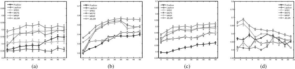
In the first group, we employ Kmeans for clustering by repeating 100 times. With different numbers of selected features, the Acc and NMI results are show in Fig. 1, Table 2 and Table 3, where the parameters are selected by grid search in a heuristic way. Other parameters, such as k and m, are empirically determined as in traditional subspace learning approaches.
As seen from Fig. 1, Table 2 and Table 3, it is clear that JELSR performs better than other approaches in most cases. Besides, although Acc and NMI are two different metrics, they both indicate the advantages of our algorithm.
In the second group, we employ another clustering algorithm, i.e., Ncut, for evaluation. On Umist data, we select s = 10 and s = 50 features. On Isolet data, we set s = 10 and s = 45 for illustration. The Acc results are in Fig. 2.
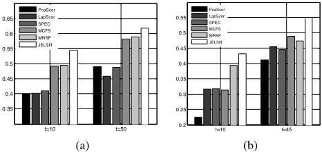
Similarly, although we employ different clustering methods, JELSR also outperforms other algorithms.
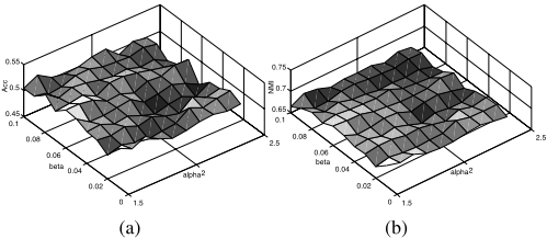
Finally, we first determine two parameters by grid search and then change them within certain ranges. The Acc results of Kmeans with different α and β are shown in Fig. 3.
As seen from Fig. 3, when two parameter are changed within a certain range, the performance of JELSR also changes within a certain range.
5 Conclusion
In this paper, we proposed a novel unsupervised feature selection algorithm. Different from traditional methods, our algorithm could combine embedding learning and sparse regression. We also provided an efficient algorithm to solve the ℓ2,1-norm regularization problem. The convergence behavior was also analyzed. Further research includes the extension of JELSR to supervised case. We will also focus on the accelerating issue of our algorithm.
| s | PcaScor | LapScor | SPEC | MCFS | MRSF | JELSR |
|---|---|---|---|---|---|---|
| s=5 | 0.5049±0.0151 | 0.4985±0.0088 | 0.4614±0.0087 | 0.5286±0.0121 | 0.5839±0.0124 | 0.6234±0.0160 |
| s=15 | 0.5337±0.0122 | 0.5178±0.0147 | 0.5191±0.0145 | 0.6260±0.0182 | 0.6142±0.0124 | 0.6515±0.0187 |
| s=25 | 0.5450±0.0132 | 0.5271±0.0152 | 0.5268±0.0152 | 0.6418±0.0204 | 0.6535±0.0167 | 0.6888±0.0204 |
| s=35 | 0.5854±0.0150 | 0.5268±0.0171 | 0.5293±0.0167 | 0.6352±0.0201 | 0.6549±0.0167 | 0.6886±0.0250 |
| s=45 | 0.6248±0.0131 | 0.5493±0.0172 | 0.5339±0.0150 | 0.6651±0.0195 | 0.6699±0.0186 | 0.6984±0.0193 |
| s | PcaScor | LapScor | SPEC | MCFS | MRSF | JELSR |
|---|---|---|---|---|---|---|
| s=5 | 0.3608±0.0047 | 0.3588±0.0047 | 0.3667±0.0048 | 0.3778±0.0055 | 0.4816 ±0.0052 | 0.5139±0.0064 |
| s=15 | 0.3813±0.0077 | 0.4971±0.0076 | 0.4958±0.0078 | 0.5769±0.0083 | 0.5736 ±0.0094 | 0.6153±0.0152 |
| s=25 | 0.5110±0.0107 | 0.5035±0.0093 | 0.5401±0.0081 | 0.6612±0.0145 | 0.6561 ±0.0106 | 0.6900±0.0155 |
| s=35 | 0.5391±0.0114 | 0.6026±0.0100 | 0.6055±0.0097 | 0.7034±0.0134 | 0.6799 ±0.0145 | 0.7272±0.0159 |
| s=45 | 0.5583±0.0115 | 0.6107±0.0099 | 0.6059±0.0098 | 0.6703±0.0146 | 0.6544 ±0.0107 | 0.7191±0.0151 |
Acknowledgement
This work is supported by NFSC, China, No. 61005003, 60975038.
@inproceedings{ijcai2011p224,
  title     = {Feature Selection via Joint Embedding Learning and Sparse Regression},
  author    = {Hou, Chenping and Nie, Feiping and Yi, Dongyun and Wu, Yi},
  booktitle = {Proceedings of the Twenty-Second International Joint Conference on
               Artificial Intelligence, {IJCAI-11}},
  publisher = {AAAI Press/International Joint Conferences on Artificial Intelligence},
  editor    = {Toby Walsh},
  pages     = {1324--1328},
  year      = {2011},
  month     = {7},
  doi       = {10.5591/978-1-57735-516-8/IJCAI11-224},
  url       = {https://doi.org/10.5591/978-1-57735-516-8/IJCAI11-224},
}
TY - CPAPER TI - Feature Selection via Joint Embedding Learning and Sparse Regression AU - Hou, Chenping AU - Nie, Feiping AU - Yi, Dongyun AU - Wu, Yi T2 - Proceedings of the Twenty-Second International Joint Conference on Artificial Intelligence, IJCAI-11 PB - AAAI Press/International Joint Conferences on Artificial Intelligence PY - 2011 SP - 1324 EP - 1328 DO - 10.5591/978-1-57735-516-8/IJCAI11-224 UR - https://doi.org/10.5591/978-1-57735-516-8/IJCAI11-224 ER -Copied
Machine-readable versions of this paper, for tools and AI agents:





