
A Fast Dual Projected Newton Method for l1-Regularized Least Squares
Proceedings of the Twenty-Second International Joint Conference on Artificial Intelligence. Pages 1275-1279.
https://doi.org/10.5591/978-1-57735-516-8/IJCAI11-216
© 2011 International Joint Conferences on Artificial Intelligence
Abstract
L1-regularized least squares, with the ability of discovering sparse representations, is quite prevalent in the field of machine learning, statistics and signal processing. In this paper, we propose a novel algorithm called Dual Projected Newton Method (DPNM) to solve the L1-regularized least squares problem. In DPNM, we first derive a new dual problem as a box constrained quadratic programming. Then, a projected Newton method is utilized to solve the dual problem, achieving a quadratic convergence rate. Moreover, we propose to utilize some practical techniques, thus it greatly reduces the computational cost and makes DPNM more efficient. Experimental results on six real-world data sets indicate that DPNM is very efficient for solving the L1-regularized least squares problem, by comparing it with state of the art methods.
- [Beck and Teboulle, 2009] A. Beck and M. Teboulle. A fast iterative shrinkage-thresholding algorithm for linear inverse problems. SIAM Journal on Imaging Sciences, 2(1):183-202, 2009.
- [Bertsekas, 1982] Dimitri P. Bertsekas. Projected new- ton methods for optimization problems with simple con- straints. SIAM Journal on Control and Optimzation, 20(2):221-246, 1982.
- [Bertsekas, 1999] Dimitri P. Bertsekas. Nonlinear Program- ming. Athena Scientific, September 1999.
- [Bishop, 2006] C.M. Bishop. Pattern recognition and ma- chine learning. Springer New York, 2006.
- [Boyd and Vandenberghe, 2004] S.P. Boyd and L. Vanden- berghe. Convex optimization. 2004.
- [Duchi and Singer, 2009] J. Duchi and Y. Singer. Efficient online and batch learning using forward backward split- ting. Journal of Machine Learning Research, 10:2899- 2934, 2009.
- [Efron et al., 2004] B. Efron, T. Hastie, I. Johnstone, and R. Tibshirani. Least Angle Regression. Analysis of Statis- tics, 32(2):407-499, 2004.
- [Figueiredo et al., 2007] M.A.T. Figueiredo, R.D. Nowak, and S.J. Wright. Gradient projection for sparse reconstruc- tion: Application to compressed sensing and other inverse problems. IEEE Journal on Selected Topics in Signal Pro- cessing, 1(4):586-597, 2007.
- [Friedman et al., 2008] J. Friedman, T. Hastie, and R. Tib- shirani. Sparse inverse covariance estimation with the graphical lasso. Biostatistics, 9(3):432, 2008.
- [Hale et al., 2007] E.T. Hale, W. Yin, and Y. Zhang. A fixed- point continuation method for ℓ 1 -regularized minimization with applications to compressed sensing. CAAM TR07-07, Rice University, 2007.
- [Kim and Park, 2010] J. Kim and H. Park. Fast Active-set- type Algorithms for ℓ 1 -regularized Linear Regression. In The 13th International Conference on Artificail Intelli- gence and Statistics, 2010.
- [Kim et al., 2007] S.J. Kim, K. Koh, M. Lustig, S. Boyd, and D. Gorinevsky. An interior-point method for large-scale ℓ 1 -regularized least squares. IEEE Journal of Selected Topics in Signal Processing, 1(4):606-617, 2007.
- [Lee et al., 2007] H. Lee, A. Battle, R. Raina, and A.Y. Ng. Efficient sparse coding algorithms. Advances in Neural Information Processing Systems, 19:801, 2007.
- [Nesterov, 1983] Y. Nesterov. A method of solving a con- vex programming problem with convergence rate O( 1 k 2 ). 27(2):372-376, 1983.
- [Schmidt et al., 2007] M. Schmidt, G. Fung, and R. Rosales. Fast optimization methods for ℓ 1 regularization: A com- parative study and two new approaches. In The 18th Eu- ropean Conference on Machine Learning, pages 286-297. Springer, 2007.
- [Tibshirani, 1996] R. Tibshirani. Regression shrinkage and selection via the lasso. Journal of the Royal Statistical Society. Series B (Methodological), 58(1):267-288, 1996.
- [Wright et al., 2009] S.J. Wright, R. Nowak, and M. Figueiredo. Sparse reconstruction by separable approximation. IEEE Transactions on Signal Processing, 57(7):2479-2493, 2009.
References were extracted automatically from the PDF and may contain errors.
Full text extracted automatically from the PDF; figures, tables and equations may differ. The PDF is the version of record.
1 Introduction
Adding an ℓ1-norm constraint or an ℓ1-norm regularization term to an optimization problem, a sparse solution can be achieved in some applications. A sparse solution usually benefits us in some aspects: good interpretation [Tibshirani, 1996] and memory savings.
The lasso [Tibshirani, 1996], a representative ℓ1regularized least squares problem 1 , has attracted more and more attentions from the field of artificial intelligence. It has a wide range of applications, such as signal reconstruction [Wright et al., 2009], image deblurring [Beck and Teboulle, 2009], gaussian graphical model structure learning [Friedman et al., 2008], sparse coding [Lee et al., 2007], curve-fitting and classification [Bishop, 2006]. In these applications, how to efficiently solve the ℓ1-regularized least squares problem becomes a critical issue. Most existing optimization methods for the ℓ1-regularized least squares problem can be broadly classified into three categories.
1 In fact, the lasso is an ℓ1-constrained least squares problem, but it can be recast as an ℓ1-regularized least squares problem under mild conditions. In the subsequent text, we only focus on the ℓ1regularized least squares problem.
First, some algorithms are designed by transforming ℓ1regularized least squares as a constrained quadratic programming problem. This is achieved by either introducing an auxiliary variable, or splitting the variable into the positive and negative parts. Representative algorithms include interior method (L1LS) [Kim et al., 2007], GPSR [Figueiredo et al., 2007] and ProjectionL1 [Schmidt et al., 2007]. However, these methods double the variable size, making the optimization more costly.
Second, several algorithms are developed in the fixedpoint-type framework: A gradient descent operation is first done, and then a soft-thresholding operation is performed. Two most representative algorithms are SpaRSA [Wright et al., 2009] and FISTA [Beck and Teboulle, 2009]. SpaRSA utilizes the Barzilai-Borwein (BB) rule [Figueiredo et al., 2007] to carefully choose the gradient descent step size. FISTA chooses the position of the soft-thresholding opearation by exploiting Nesterov's method [Nesterov, 1983]. Some other fixed-point-type algorithms include FOBOS [Duchi and Singer, 2009], fixed point continuation [Hale et al., 2007], etc. However, these algorithms are first-order methods, not utilizing the second-order information.
Third, a few active-set-type algorithms are studied. A very recent method, called block principal pivoting (BP) [Kim and Park, 2010] is proposed to solve the ℓ1-regularized least squares problem. It's a further development based on least angle regression (LARS) [Efron et al., 2004] and feature-sign (FS) search algorithm [Lee et al., 2007]. Kim and Park [2010] give a dual problem and then utilize it to obtain KKT conditions. Subsequently, BP is built based on the KKT conditions. However, BP doesn't directly solve the dual problem, since the constraint of the dual problemmake it difficult to design a very efficient algorithm (see Section 2.3).
Although various methods mentioned above are designed to solve the ℓ1-regularized least squares problem, none of them reports a quadratic convergence rate 2 . In this paper, we propose a second-order algorithm called Dual Projected Newton Method (DPNM) to efficiently solve the ℓ1-regularized least squares problem. By skillfully introducing an auxiliary variable and exploiting the characteristic of the ℓ1-norm,
2 The quadratic convergence rate here refers to limk→∞||xk+1
-
x⋆ ||/||xk -x⋆ ||2 = μ with μ > 0. It achieves a δ-accurate solution
x (||x - x⋆ || ≤ δ) in O(log log(1/δ)) steps.
we derive a new dual formulation of the ℓ1-regularized least squares as a box constrained quadratic programming problem. Due to the simple box constraint in our new dual problem, a projected Newton method is used to solve the dual problem, achieving a quadratic convergence rate. Moreover, we apply some practical techniques to DPNM, greatly reducing the cost per iteration. In the sequel, we will see that the new dual form we derive doesn't increase the variable size, although we introduce an auxiliary variable. Low computational cost per iteration and less iterative steps make DPNM quite efficient. Empirical studies demonstrate that DPNM converges much faster than several state of the art algorithms by comparing the CPU time consumed.
The remainder of this paper is organized as follows. In Section 2, we present the Dual Projected Newton Method (DPNM) in detail. In Section 3, experimental results are shown on six real-world data sets. Concluding remarks are given in Section 4.
2 Dual Projected NewtonMethod
2.1 Notations
First of all, we introduce some notations in this paper. Scalars are denoted by lower case letters (e.g., x ∈ R) and vectors by lower case bold face letters (e.g., x ∈ Rn). xi denotes the i-th element of a vector x. Matrix and Sets are denoted by capital letters (e.g., A, I) and ♯(I ) indicates the number of elements in the set I. AI denotes a submatrix of A, containing the corresponding rows and columns indexed by I, and xI denotes a sub-vector of x including the corresponding elements indexed by I. ℓ1, ℓ2 and ℓ∞ norms of x are respectively denoted by ||x||1 = ∑ni=1 |xi|, ||x||2 = √∑ni=1 x2i and ||x||∞ = maxni=1 |xi|. x⊙y(x, y ∈ Rn) is the elementwise product of x and y. y = sign(x) ⇔ ∀i, yi = sign(xi) and y = |x| ⇔ ∀i, yi = |xi|.
2.2 Problem Statement
The ℓ1-regularized least squares problem is formulated as the following optimization problem:
where A = [aT1 ; · · · ; aTm](ai ∈ Rn, i = 1, · · · ,m) is an m× n data matrix; b is a regression vector; τ is a tradeoff parameter. In this paper, we focus on the case of m ≥ n, in which we assume AT A has full rank. This assumption is also introduced by Kim and Park [2010] when their BP algorithm is proposed. The full rank assumption is usually reasonable in practical applications. For instance, in the polynomial curve-fitting problem [Bishop, 2006], the number of samples is usually larger than the order of the polynomial, in which AT A has full rank. In the classification task, each row of A is a sample and bi is the corresponding label. When the data is large-scale but not so high dimensional, the assumption that AT A has full rank usually holds. Moreover, in the waveletbased image deblurring problems [Beck and Teboulle, 2009], AT A always has full rank. Besides, in the gaussian graphical model structure learning problem [Friedman et al., 2008], the ℓ1-regularized least squares is a subproblem, in which the full rank assumption is satisfied.
2.3 Dual Problem of ℓ1-regularized Least Squares
In this subsection, we derive a new dual problem of Eq. (1). By introducing an auxiliary variable y, we reformulate Eq. (1) as the following constrained optimization problem:
We show in the following proposition that this constrained optimization problem holds the strong duality property.
Proposition 1 Strong duality of Eq. (2) holds.
Proof Let In and Om×n be an n × n identity matrix and an m× n zero matrix, respectively. Denote
Then, Eq. (2) can be equivalently formulated as follows:
The objective function in Eq. (4) is convex and the affine equality constraint satisfies Slater's condition [Boyd and Vandenberghe, 2004]. Therefore, the strong duality of Eq. (4) holds and so does Eq. (2). □
Proposition 1 inspires us to solve the dual problem of Eq. (2). Let μ be the Lagrange multiplier corresponding with the equality constraint and we get the Lagrange function as follows:
By minimizing Eq. (5) with respect to the primal variables x, y, we obtain the dual objective function as follows:
Based on the dual norm introduced in [Boyd and Vandenberghe, 2004], we obtain
Then, by maximizing Eq. (6) with respect to the dual variable μ, we get the dual problem as follows:
where H = (AT A)-1 and const is a constant term. We convert the above maximum problem to the following minimum problem by inverting the sign of ˜D(μ) and omitting the constant term:
Now, we have transformed the non-differentiable ℓ1regularized least squares problem into a quadratic programming problem with a simple box constraint, which is essential to design an efficient optimization algorithm. We should mention that the dual problem is still an optimization problem over an n-dimensional vector space, although we introduce an auxiliary variable. If we can efficiently obtain the optimal solution μ⋆ of dual problem Eq. (9), then we get the optimal solution of the primal problemEq. (1) via
As a matter of fact, before our new dual problem, some literatures [Kim et al., 2007; Wright et al., 2009; Kim and Park, 2010] have given the following dual problem:
The constraint in Eq. (11) is more complex than the constraint in Eq. (9), since AT α makes all the components (i.e., αis) of α coupled with each other, hence developing an efficient algorithm to solve Eq. (11) is not so easy. Thus, fewer algorithm is designed by solving the dual problem Eq. (11) directly. Kim et al. [2007] and Wright et al. [2009] use Eq. (11) to obtain the duality gap and some other properties. Kim and Park [2010] exploit Eq. (11) to get KKT conditions, but not directly solve it. However, the box constraint in Eq. (9) indicates that the components of μ aren't coupled with each other, which is a very good property for designing an efficient algorithm.
2.4 Algorithm
We design an efficient algorithm called Dual Projected Newton Method (DPNM) to solve the dual problem Eq. (9). Generally speaking, Eq. (9) can be solved by a projected gradient method [Bertsekas, 1999], that is, generating a sequence {μk } by μk+1 = [μk -ηk∇D(μk )]+, where [x]+ = sign(x) ⊙min(τ, |x|) is the Euclidean projection of x onto the box constraint in Eq. (9). However, the convergence rate of the projected gradient method is at most linear. Subsequently, we focus on the following iterations by incorporating the idea of Newton's method, aiming to achieve a quadratic convergence rate:
where M k is a positive definite matrix containing the secondorder information and ηk is a step size. How to choose the positive definite matrix M k is quite critical to the performance of an algorithm. In the unconstrained optimization problem, M k can be simply chosen as the inverse of the Hessian matrix, but Bertsekas [1982] shows that, in the constrained optimization problem, choosing M k as the inverse of Hessian matrix can't guarantee objective descent per iteration, even can't guarantee convergence. In the case of simple constraints (e.g., box constraint), Bertsekas [1982] suggests a class of matrices M k for which objective descent and convergence can be guaranteed.
In the framework of [Bertsekas, 1982], we propose the projected Newton method to solve the dual problem Eq. (9) and we prove in the sequel that the convergence rate is at least quadratic. Define
where ϵk = min(||μk - [μk - ∇D(μk )]+||2, ϵ) and ϵ is a small positive scalar. Denote
Then, we obtain the following proposition:
Proposition 2 H k is a positive definite matrix.
Proof ∀ x ∈ Rn, x ̸= 0,
where ¯xi = xi, if i /∈ I k , 0 otherwise. Under the assumption that AT A has full rank, we get that H is positive definite. Then Hii > 0, ∑i∈I k Hiix2i ≥ 0 and ¯xT H¯x ≥ 0. We note that x ̸= 0, so at least one of ∑i∈I k Hiix2i and ¯xT H¯x is strictly positive. Thus, xT H k x > 0 is satisfied and the proposition is verified. □
In our method, M k is chosen as M k = (H k )-1 , satisfying the condition that M k is a positive definite matrix. Denote
The step size ηk is chosen as ηk = αmk with α ∈ (0, 1), satisfying mk is the first nonnegative integer m such that
where σ is a constant. Then μk+1 is given by μk+1 = [μk - ηk pk ]+. The detailed procedure of DPNM is listed in Algorithm 1. Next, we declare that Algorithm 1 not only guarantees convergence, but also has a quadratic convergence rate in the following theorem.
Theorem 1 The sequence {μk } generated by Algorithm 1 converges to the optimal solution μ⋆ and the convergence rate of {||μk -μ⋆ ||2} is at least quadratic.
Proof The objective functionD(μ) in Eq. (9) is twice continuously differentiable and the Hessian matrix ∇2D(μ) = H is positive definite under the assumption that AT A has full rank. Therefore, the objective function D(μ) is convex and Eq. (9) has a unique solution μ⋆ . Furthermore, there exists positive scalars λ1, λ2 (λ1 and λ2 are the smallest and largest eigenvalues of the Hessian matrix respectively.) such that λ1||z||22 ≤ zT ∇2D(μ)z ≤ λ2||z||22 for any z ∈ Rn. According to the KKT conditions [Bertsekas, 1999], ∂D(μ⋆ ) ∂μi > 0, if
Algorithm 1: DPNM-Dual Projected Newton Method
Input : A ∈ Rm×n, b ∈ Rn, τ ∈ R, μ0 ∈ Rn 1 Initialize σ = 10-3; α = 0.5; ϵ = 10-4; 2 Compute H = (AT A)-1 ; Atb = AT b; 3 for k = 0, 1, · · · do 4 wk = ||μk - [μk - ∇D(μk )]+||2; 5 ϵk = min(wk , ϵ); 6 Compute I k by Eq. (13); 7 Compute pk , μk (ηk ) by Eq. (16); 8 m= 0; 9 while Eq. (17) is not satisfied do 10 m = m + 1; ηk = αm; 11 end 12 μk+1 = [μk - ηk pk ]+; 13 if convergence criterion is satisfied then 14 iter = k + 1; break; 15 end 16 end 17 μ⋆ = μk+1 ; x⋆ = H (Atb - μ⋆); Output: μ⋆ , x⋆ , iterμ⋆i = -τ; ∂D(μ⋆ ) ∂μi < 0, if μ⋆i = τ. Obviously, ∇2D(μ) = H is Lipschitz continuous. Based on the properties above and the Proposition 4 (and its extensions) in [Bertsekas, 1982], Algorithm 1 converges to the optimal solution μ⋆ and the convergence rate of {||μk -μ⋆ ||2} is at least quadratic. □
The quadratic convergence rate is remarkable, which indicates that Algorithm 1 can achieve a δ-accurate solution μ (||μ-μ⋆ ||2 ≤ δ) for Eq. (9) in O(log log(1/δ)) steps.
2.5 Implementation Details
We present the implementation details of Algorithm 1, in which some practical techniques are utilized to reduce the cost per iteration.
- Since H and Atb are used several times in Algorithm 1, they can be computed when we initialize the algorithm, which greatly reduces the computational time. Here O(n3 ) operations are needed and we focus on the problem where n is not very large.
- The computational bottleneck in Algorithm 1 is for computing pk in Eq. (16), which requires an inverse operation for an n × n matrix H k . But in fact, we only need to compute the inverse of a smaller r × r matrix, where r = n - ♯(I k ). Denote
Then there exists a permutation matrix P such that
Therefore,
- We note that
To further reduce the computational cost, the inverse and multiplication operation H -1 ˜ I k ∇D(μk ) ˜ I k can be replaced by the Cholesky decomposition, which can be efficiently obtained requiring O(r3 ) (r < n) operations. Moreover, BI k is a diagonal matrix, B-1 I k ∇D(μk )I k requires only O(n - r) operations.
- P is a permutationmatrix, which indicates that PH k P T in Eq. (20) is just the permutation of the rows and columns for H k , according to the index sets ˜ I k and I k , without requiring any multiplication operation. This conclusion can be also applied to Eq. (22).
3 Experiments
3.1 Experimental Settings
All algorithms in the experiments are implemented in Matlab and they are tested on six real-world data sets: Extended Yale Face Database B (ExtYaleB), USPS, Yale Face Database B (YaleB), PIE, Isolet and dna. Their basic information is listed in Table 1 (m is the number of samples and n is the dimension. ExtYaleB and YaleB are respectively resized to 32 × 32 and 40 × 30.).
In the experiments, every row of A is a sample in each data set and bi is the corresponding label. For the ℓ1-regularized least squares problem in Eq. (1), the optimal solution x⋆ equals 0 if τ ≥ ||AT b||∞ [Wright et al., 2009]. In order to avoid a trivial solution, we set τ = tol × ||AT b||∞ with different tols (tol = 10-1, 10-2, 10-3, 10-4, 10-5 ).
To demonstrate the effectiveness and efficiency of DPNM, we compare DPNM with four state of the art methods: BPR 3 [Kim and Park, 2010], L1LS 4 [Kim et al., 2007], FISTA 5 [Beck and Teboulle, 2009] and SpaRSA 6 [Wright et al., 2009]. BPR is an active-set-type algorithm based on obtaining KKT conditions from Eq. (11). L1LS, FISTA and SpaRSA directly solve the ℓ1-regularized least squares problem in Eq. (1). Since different algorithms have different terminated criteria, for fair comparisons, we first run the L1LS algorithm until its relative duality gap is less than or equal to 10-4 and then record its objective value P ⋆ in Eq. (1). We next run DPNM, SpaRSA, FISTA and BPR until the objective value in Eq. (1) are less than or equal to P ⋆, or the iterative steps exceeds 10000. We independently run the five algorithms 10 times respectively with different random starting points. To further speed up SpaRSA and FISTA algorithms, the continuation technique [Hale et al., 2007] is adopted.
3 BPR is an improved algorithm based on BP.
4 http://www.stanford.edu/˜boyd/l1_ls/
5 http://www.eecs.berkeley.edu/˜yang/
software/l1benchmark/
6 http://www.lx.it.pt/˜mtf/SpaRSA/
| data | size | coeff | average time(CPU | seconds) | ♯ average | ||||||||
|---|---|---|---|---|---|---|---|---|---|---|---|---|---|
| set | m×n | tol | DPNM | BPR | L1LS | FISTA | SpaRSA | DPNM | BPR | iterations L1LS | FISTA | SpaRSA | |
| ExtYaleB | 2414 × 1024 | 10-1 | 0.9062 | 2.0817 | 8.7543 | 18.3742 | 2.9490 | 15.0 | 83.0 | 46.0 | 3258.7 | 526.5 | |
| 10-2 | 1.0378 | 0.8750 | 26.8962 | 42.9980 | 6.0558 | 18.0 | 16.0 | 35.0 | 8037.7 | 1082.1 | |||
| 10-3 | 0.4971 | 1.0604 | 92.1205 | 49.8914 | 8.5170 | 10.0 | 10.0 | 37.0 | 10000.0 | 1564.3 | |||
| 10-4 | 0.2746 | 1.6095 | 279.9859 | 50.1130 | 55.3159 | 3.0 | 9.0 | 38.0 | 10000.0 | 10001.0 | |||
| 10-5 | 0.2710 | 2.1223 | 325.1329 | 50.1931 | 57.0251 | 2.0 | 10.0 | 30.0 | 10000.0 | 10001.0 | |||
| Isolet | 7797 × 617 | 10-1 | 0.3560 | 2.2915 | 3.1007 | 0.6595 | 0.5114 | 12.0 | 53.0 | 33.0 | 31.6 | 36.2 | |
| 10-2 | 0.2544 | 0.9970 | 15.3178 | 1.2751 | 0.9600 | 8.0 | 12.0 | 54.0 | 92.2 | 79.9 | |||
| 10-3 | 0.2031 | 1.1891 | 21.0388 | 3.3981 | 4.9525 | 6.0 | 9.0 | 35.0 | 283.0 | 412.0 | |||
| 10-4 | 0.1649 | 2.0951 | 29.2915 | 14.3518 | 86.9161 | 3.0 | 11.0 | 37.0 | 1323.6 | 7098.0 | |||
| 10-5 | 0.1513 | 1.8817 | 31.0686 | 47.2366 | 123.6213 | 1.0 | 9.0 | 32.0 | 4400.4 | 10001.0 | |||
| PIE | 11154 × 1024 | 10-1 | 1.2425 | 126.5265 | 91.2420 | 74.9511 | 7.8936 | 14.0 | 720.0 | 115.0 | 2687.0 | 251.0 | |
| 10-2 | 1.0813 | 3.0447 | 106.5602 | 204.9801 | 7.0325 | 11.0 | 14.0 | 70.0 | 7428.6 | 219.7 | |||
| 10-3 | 0.9106 | 3.7257 | 206.4877 | 275.4339 | 28.7151 | 10.0 | 10.0 | 32.0 | 10000.0 | 956.0 | |||
| 10-4 | 0.5900 | 5.3669 | 1332.5470 | 275.4096 | 287.1595 | 3.0 | 9.0 | 62.0 | 10000.0 | 9374.9 | |||
| 10-5 | 0.5598 | 7.1639 | 1463.5147 | 275.4168 | 320.7441 | 1.0 | 10.0 | 35.0 | 10000.0 | 10001.0 | |||
| USPS | 7291 × 256 | 10-1 | 0.0617 | 0.2466 | 1.9089 | 0.2585 | 0.1741 | 8.0 | 11.0 | 28.0 | 57.9 | 33.6 | |
| 10-2 | 0.0595 | 0.3149 | 3.9277 | 0.7283 | 0.2934 | 6.0 | 10.0 | 25.0 | 212.3 | 57.2 | |||
| 10-3 | 0.0421 | 0.3917 | 5.2646 | 0.7591 | 0.7786 | 4.0 | 9.0 | 18.0 | 227.1 | 166.8 | |||
| 10-4 | 0.0432 | 0.4112 | 5.2152 | 2.8532 | 21.6712 | 2.0 | 8.0 | 12.0 | 930.2 | 4504.2 | |||
| 10-5 | 0.0372 | 0.4825 | 6.5782 | 10.2410 | 48.6217 | 1.0 | 9.0 | 12.0 | 3251.0 | 10001.0 | |||
| YaleB | 5850 × 1200 | 10-1 | 2.8930 | 62.8636 | 28.9774 | 58.9738 | 4.7258 | 26.0 | 968.0 | 39.0 | 3443.2 | 256.5 | |
| 10-2 | 1.8639 | 2.7727 | 81.4151 | 169.9488 | 20.0788 | 18.0 | 22.0 | 43.0 | 10000.0 | 1162.1 | |||
| 10-3 | 1.7421 | 2.9562 | 139.2338 | 170.2495 | 33.2614 | 17.0 | 19.0 | 32.0 | 10000.0 | 2017.5 | |||
| 10-4 | 0.9744 | 2.7449 | 378.8279 | 169.9587 | 155.3790 | 10.0 | 11.0 | 26.0 | 10000.0 | 9052.3 | |||
| 10-5 | 0.6419 | 3.4733 | 1295.9871 | 169.7176 | 185.0566 | 6.0 | 9.0 | 41.0 | 10000.0 | 10001.0 | |||
| dna | 3186 × 180 | 10-1 | 0.0135 | 0.0776 | 0.3058 | 0.0255 | 0.0172 | 2.0 | 7.0 | 22.0 | 23.6 | 17.0 | |
| 10-2 | 0.0158 | 0.0826 | 0.4766 | 0.0424 | 0.0363 | 2.0 | 6.0 | 23.0 | 58.7 | 43.8 | |||
| 10-3 | 0.0164 | 0.0871 | 0.5249 | 0.0956 | 0.0660 | 2.0 | 6.0 | 17.0 | 184.3 | 82.4 | |||
| 10-4 | 0.0138 | 0.0879 | 0.3110 | 0.1936 | 0.0904 | 1.0 | 6.0 | 17.0 | 431.3 | 121.4 | |||
| 10-5 | 0.0161 | 0.0832 | 0.2097 | 0.4012 | 0.1061 | 1.0 | 6.0 | 13.0 | 920.6 | 140.3 | |||
3.2 Experimental Analysis
The average computational time (The time of computing H and Atb for DPNM is also included.) and the average number of iterations over 10 independent executions (with different random starting points) are listed in Table 1. From these results, we can get: (a) DPNM is the most efficient among all the algorithms, both on CPU time and iterative steps, especially for small τs. (b) The CPU time (iterative steps) for DPNM tends to become less when the regularization parameter τ decreases. When τ is small, the feasible region in Eq. (9) becomes small. Thus, it's easier and cheaper to find the optimal solution in a smaller feasible region. On the contrary, L1LS, FISTA and SpaRSA tends to consume more CPU time and iterative steps when τ becomes smaller and this phenomenon can be also observed in [Wright et al., 2009]. For BPR, not such an obvious phenomenon is observed. On some data sets (e.g., PIE and YaleB), when τ = 10-1 × ||AT b||∞, the iterative steps and CPU time are very large, which indicates that BPR is not so stable when the regularization τ varies. This is due to the frequent variables exchanging among different groups. (c) For BPR, sometimes less iterative steps even leads to more CPU time. The computational cost for BPR varies greatly for each iteration, more iterative steps with cheaper cost per-iteration consuming less CPU time is possible. (d) Most of the time, the iterative steps for L1LS are much smaller than that for SpaRSA and FISTA, but the CPU time is more, since the computational cost per iteration for L1LS is more expensive than SpaRSA and FISTA. Whereas too large iterative steps for SpaRSA and FISTA make them less efficient than DPNM and BPR. (e) L1LS, SpaRSA and FISTA are very slow when τ is small, although continuation technique [Hale et al., 2007] is adopted for SpaRSA and FISTA. For DPNM, the CPU time consumed doesn't vary too much when τ changes.
To further understand the accuracy of the solutions for different algorithms, we plot the average objective values of Eq. (1) for the five algorithms on the six real-world data sets as in Figure 1. From the figures, we can see that BPR and DPNM achieve the smallest objective values and they are very competitive most of the time. In Table 1, we find the iterative steps of SpaRSA and FISTA sometimes exceed 10000, which indicate that their objective values might be still larger than P ⋆ when the iterative steps reach 10000. Integrating Table 1 and Figure 1 together, we can see that when an algorithm's iterative steps exceed 10000, the corresponding objective value is truly larger than L1LS's objective value P ⋆, which confirms that our conclusion is correct.
In all, DPNM is very efficient and effective for solving the ℓ1-regularized least squares problem: DPNM converges fast with an at least quadratic convergence rate, which requires tol tol only a dozen even fewer steps, and consumes much less CPU time.
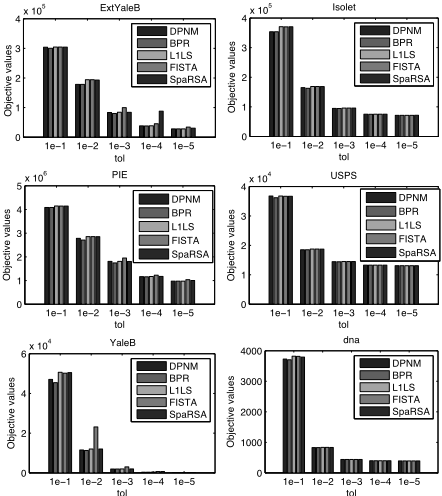
Figure 1: The bar plots of average objective values in Eq. (1) for different algorithms. Each subfigure shows the average objective value vs. tol bar on a real-world data set.
4 Conclusions
In this paper, a novel algorithm called DPNM is proposed to efficiently solve the ℓ1-regularized least squares problem. Our main contribution is reflected in: (1) We derive a new dual form of the ℓ1-regularized least squares as a box constrained quadratic optimization problem. (2) Due to the simple box constraint, a projected Newton method is applied to efficiently solve the new dual problem, achieving a quadratic convergence rate. Empirical studies on six real-world data sets demonstrate that DPNM is more efficient than several state of the art algorithms. A limitation of DPNM is that it works under the assumption that AT A has full rank, and so does BPR. Whereas the other three algorithms (L1LS, FISTA, SpaRSA) can still work without the full rank assumption. In our future work, we will extend DPNM to the case without the full rank assumption.
Acknowledgments
This work is supported by NSFC (Grant No. 61075004 and No. 60835002).
@inproceedings{ijcai2011p216,
  title     = {A Fast Dual Projected Newton Method for l1-Regularized Least Squares},
  author    = {Gong, Pinghua and Zhang, Changshui},
  booktitle = {Proceedings of the Twenty-Second International Joint Conference on
               Artificial Intelligence, {IJCAI-11}},
  publisher = {AAAI Press/International Joint Conferences on Artificial Intelligence},
  editor    = {Toby Walsh},
  pages     = {1275--1279},
  year      = {2011},
  month     = {7},
  doi       = {10.5591/978-1-57735-516-8/IJCAI11-216},
  url       = {https://doi.org/10.5591/978-1-57735-516-8/IJCAI11-216},
}
TY - CPAPER TI - A Fast Dual Projected Newton Method for l1-Regularized Least Squares AU - Gong, Pinghua AU - Zhang, Changshui T2 - Proceedings of the Twenty-Second International Joint Conference on Artificial Intelligence, IJCAI-11 PB - AAAI Press/International Joint Conferences on Artificial Intelligence PY - 2011 SP - 1275 EP - 1279 DO - 10.5591/978-1-57735-516-8/IJCAI11-216 UR - https://doi.org/10.5591/978-1-57735-516-8/IJCAI11-216 ER -Copied
Machine-readable versions of this paper, for tools and AI agents:





