
Learning Decision Rules from Data Streams
Proceedings of the Twenty-Second International Joint Conference on Artificial Intelligence. Pages 1255-1259.
https://doi.org/10.5591/978-1-57735-516-8/IJCAI11-213
© 2011 International Joint Conferences on Artificial Intelligence
Abstract
Decision rules, which can provide good interpretability andflexibility for data mining tasks, have received very littleattention in the stream mining community so far. In this workwe introduce a new algorithm to learn rule sets, designed for open-ended data streams.The proposed algorithm is able to continuously learn compact ordered and unordered rule sets. The experimental evaluation shows competitive results in comparison with VFDT and C4.5rules.
- Adä, I. and M. R. Berthold (2010). The new iris data: modu- lar data generators. In KDD, pp. 413-422.
- Clark, P. and T. Niblett (1989). The CN2 induction algorithm. Machine Learning 3, 261-283.
- Cohen, W. (1995). Fast effective rule induction. In Proceed- ings of the ICML, 115-123.
- Morgan Kaufmann.
- Domingos, P. (1996). Unifying instance-based and rule-based induction. Machine Learning 24, 141-168.
- Ferrer, F., J. Aguilar, and J. Riquelme (2005). Incremen- tal rule learning and border examples selection from nu- merical data streams. Journal of Universal Computer Sci- ence 11(8), 1426-1439.
- Frank, E. and I. H. Witten (1998). Generating accurate rule sets without global optimization. In Proceedings of ICML, pp. 144-151.
- Morgan Kaufmann.
- Gama, J., R. Fernandes, and R. Rocha (2006). Decision trees for mining data streams. Intelligent Data Analysis 10(1), 23-46.
- Gama, J., R. Rocha, and P. Medas (2003). Accurate decision trees for mining high-speed data streams. In Proceedings of KDD, pp. 523-528. ACM Press.
- Gama, J., R. Sebastião, and P. P. Rodrigues (2009). Issues in evaluation of stream learning algorithms. In Proceedings of KDD, pp. 329-338.
- Kolter, J. Z. and M. A. Maloof (2003). Dynamic weighted majority: A new ensemble method for tracking concept drift. In Proceedings of ICDM, pp. 123-130. IEEE Com- puter Society.
- Maloof, M. and R. Michalski (2004). Incremental learning with partial instance memory. Artificial Intelligence 154, 95-126.
- Quinlan, R. (1993). C4.5: Programs for Machine Learning.
- Rivest, R. (1987). Learning Decision Lists. Machine Learn- ing 2, 229-246.
- Schlimmer, J. C. and R. H. Granger (1986). Incremental learning from noisy data. Machine Learning 1, 317-354.
- Street, W. N. and Y. Kim (2001). A streaming ensemble al- gorithm SEA for large-scale classification. In Proceedings KDD, pp. 377-382. ACM Press.
- Wang, H., W. Fan, P. S. Yu, and J. Han (2003). Mining concept-drifting data streams using ensemble classifiers. In Proceedings of KDD, pp. 226-235. ACM Press.
- Weiss, S. and N. Indurkhya (1998). Predictive Data Mining, a practical Guide. Morgan Kaufmann Publishers.
- Widmer, G. and M. Kubat (1996). Learning in the presence of concept drift and hidden contexts. Machine Learning 23, 69-101.
References were extracted automatically from the PDF and may contain errors.
Full text extracted automatically from the PDF; figures, tables and equations may differ. The PDF is the version of record.
1 Motivation
Large decision trees are difficult to understand because each node appears in a specific context established by the outcomes of tests at the antecedent nodes. The work of Rivest (1987) presents a new representation, decision lists, that generalizes decision trees. The advantage of this representation is modularity and consequently interpretability: each rule is independent of the others, and can be interpreted in isolation of the others.
Rule sets take advantage of not being hierarchically structured, so concept descriptions can be updated or removed when becoming out-of-date without hardly affecting the learning efficiency. A decision rule is a logic predicate of the form IF antecedent THEN label. The antecedent is a conjunction of conditions of the form Attribute ⊗ Values, and ⊗ is a operator that states a relation between a particular attribute and values of its domain. Contrary to partitions obtained with decision tree based approaches, the regions given by decision rules do not model the whole space. Thus, new test examples may not be covered by any rule.
2 RelatedWork
A widely used strategy consists of building decision lists from decision trees, as it is done in Quinlan (1993). In any decision tree when a case reaches a leaf, the conditions that must be satisfied appear along the path from the root to the leaf. So, any tree can be easily transformed into a collection of rules. Each rule corresponds to the path from the root to a leaf, and there are as many rules as leaves. This process generates a set of rules with the same complexity as the decision tree. However, it has been shown that the antecedents of individual rules may contain irrelevant conditions. C4.5rules (Quinlan, 1993) uses an optimization procedure to simplify conditions. The optimization is done in two phases. First, each rule is generalized by deleting conditions that do not seem to be helpful in discriminating the classes. A greedy search method is used. At each step the rule is evaluated as if one condition was dropped. The condition that produces the lowest increase of the pessimistic estimate of the error rate of the rule is eliminated. The pessimistic error rate is estimated similarly to the process discussed in the pruning phase of C4.5. After generalizing individual rules some of them may become identical to others, and so the duplicates are removed. Also, some of them may have no conditional part. They are also removed. In the second phase, all rules are grouped by the predicted class. For each class, the set of rules is simplified by removing rules whose removal does not diminish the accuracy of the complete set. Empirical studies (Quinlan, 1993) have shown that the set of rules is both simpler and more accurate than the initial tree. Frank and Witten (1998) present a method for generating rules from decision trees without using global optimization. The basic idea is to generate a decision tree in a breadth-first order, select the best rule, remove the examples covered by the rule and iteratively induce further rules for the remaining instances.
Several algorithms appear in literature for building decision lists (Rivest, 1987; Clark and Niblett, 1989; Cohen, 1995; Domingos, 1996; Weiss and Indurkhya, 1998). As pointed out by Wang et al. (2003), a drawback of decision trees is that even a slight drift of the target function may trigger several changes in the model and severely compromise learning efficiency. On the other hand, ensemble methods avoid expensive revisions by weighting the members, but may run the risk of building unnecessary learners when virtual drifts are present in data.
Fundamental incremental rule learners include STAGGER (Schlimmer and Granger, 1986), the first system designed expressly for coping with concept drift, the FLORA family of algorithms (Widmer and Kubat, 1996) with FLORA3 being the first system able to deal with recurring contexts, and the AQ-PM family (Maloof and Michalski, 2004). The most representative algorithm is the AQ11-PM system (Kolter and Maloof, 2003; Maloof and Michalski, 2004). It selects positive examples from the boundaries of its rules (hyperrectangles) and stores them in memory. When new examples arrive, AQ11-PM combines them with those held in memory, applies the AQ11 algorithm to modify the current set of rules, and selects new positive examples from the corners, edges, or surfaces of such hyper-rectangles (extreme examples). Since pure incremental rule learners store in memory every training example, many of them have not still adapted to a data streams environment, especially those featuring numerical attributes.
Decision Rules from Data Streams. At our best knowledge, the work of Ferrer, Aguilar, and Riquelme (2005) is the only streaming rule learner published till now. In that work, the authors present system Facil, a classification system based on decision rules that may store up-to-date border examples to avoid unnecessary revisions when virtual drifts are present in data. Consistent rules classify new test examples by covering and inconsistent rules classify them by distance as the nearest neighbor algorithm. Similarly to AQPM, Facil uses a forgetting mechanism that can be either explicit or implicit. Explicit forgetting takes places when the examples are older than a user defined threshold. Implicit forgetting is performed by removing examples that are no longer relevant as they do not enforce any concept description boundary. The core of this approach is that rules may be inconsistent by storing positive and negative examples which are very near one another (border examples). A rule is said consistent when does not cover any negative (different label) example. The aim is to seize border examples up to a threshold is reached. This threshold is given as an user parameter and sets the minimum purity of a rule. The purity of a rule is the ratio between the number of positive examples that it covers and its total number of covered examples, positive and negative. When the threshold is reached, the examples associated with the rule are used to generate new positive and negative consistent rules. A restriction in Facil is that it requires normalized (between 0 and 1) numerical data.
3 Rule Learning fromData Streams
In this section we present the Very Fast Decision Rules algorithm. VFDR is designed for high-speed data streams. It is a single pass algorithm, that learns ordered and/or unordered rules.
The algorithm begin with a empty rule set (RS), and a default rule {} → L, where L is initialized to ∅. L is a data structure that contains information used to classify test instances, and the sufficient statistics needed to expand the rule. Each rule (r) learned is a conjunction of literals, that are conditions based on attribute values, and a Lr. For numerical attributes, each literal is of the form ati > v, or ati ≤ v for some feature ati and some constant v. For categorical attributes VFDR produce literals of the form ati = vj where vj is a value in the domain of ati.
Growing a set of rules. If all the literals are true for a given example, then the example is said to be covered by the rule. The labeled examples covered by a rule are used to update Lr. A rule is expanded with the literal that minimizes the entropy of the class labels of the examples covered by the rule. Lr accumulates the sufficient statistics to compute the entropy of all possible literals. Lr is a data structure that contains: an integer, that stores the number of examples covered by the rule; a vector, to compute p(ci), the probability of observing examples of class ci; a matrix p(ati = vj |ci), to compute the probability of observing value vj of a nominal attribute ati, per class; and a btree to compute the probability of observing values greater than vj of continuous attribute ati, p(ati > vj|ci), per class. The information maintained in Lr is similar to the sufficient statistics in VFDT like algorithms. Gama et al. (2006) presents efficient algorithms to maintain Lr. The main difference, is that instead of selecting the attribute with best information gain considering all the partitions based on the attribute values, it selects the condition (ati = vj, ati ≤ vj, or ati > vj) that minimizes the entropy of the class distribution in the corresponding partition.
The sample size to decide when to expand a rule is given by Hoeffding bound. It guarantees that with the probability 1 - δ the true mean of a random variable x with a range R will not differ from the estimated mean after n independent observations by more than: ϵ = √ R2 ln(1/δ) 2n . In order to learn decision rule lists, Hoeffding bound determines the number of observations after which a rule can be expanded or new rule can be induced. It is not efficient to check for the sufficient number of examples with every incoming example, therefore it is done after only Nmin observations.
The set of rules (RS) is learned in parallel, as described in Algorithm 1. We consider two cases: learning ordered or unordered set of rules. In the former, every labeled example updates statistics of the first rule that covers it. In the latter, every labeled example updates statistics of all the rules that covers it. If a labeled example is not covered by any rule, the default rule is updated.
The expansion of a rule is done with Algorithm 2 that employs the aforementioned Hoeffding bound. For each attribute Xi, the value of split evaluation function H is computed for each attribute value vj , which was observed in more than 10% of examples. If the best split hbest is better than not splitting, i.e. satisfies condition h0 - hbest > ϵ the rule, is expanded with condition Xa = vj and class of the rule is assigned according to the majority class of observations of Xa = vj .
Classification strategies. Assume that a rule r covers a test example. The example will be classified using the information in Lr of that rule. The simplest strategy uses the distribution of the classes stored in Lr, and classify the example in the class that maximizes p(ci). This strategy only use the information about class distributions and does not look for the attribute-values. It uses only a small part of the available information, a crude approximation to the distribution of the examples. In a more informed strategy, a test example is classified with the class that maximizes the posteriori probability given by Bayes rule assuming the independence of the attributes given the class. There is a simple motivation for this option. L stores information about
Algorithm 1: VFDR: Rule Learning Algorithm.
input : S: Stream of examples Nmin: Minimum number of examples ordered set: boolean flag output: RS: Set of Decision Rules begin Let RS ← {} Let default rule L ← ∅ foreach example (x, yk) ∈ S do foreach Rule r ∈ RS do if r covers the example then Update sufficient statistics of Rule r if Number of examples in Lr > Nmin thenr ← ExpandRule(r) if ordered set then BREAK if none of the rules in RS trigger then Update sufficient statistics of the empty rule if Number of examples in L > Nmin then RS ← RS∪ ExpandRule(default rule)the distribution of the attributes given the class usually for hundreds or even thousands of examples, before expanding the rule and re-initializing the counters. Naive Bayes takes into account not only the prior distribution of the classes, but also the conditional probabilities of the attribute-values given the class. This way, there is a much better exploitation of the available information in each rule. Given the example ⃗x = (x1, . . . , xj) and applying Bayes theorem, we obtain: P (ck |⃗x) ∝ P (ck) ∏ P (xj |ck).
Using naive Bayes in VFDT like algorithms, is a wellknown technique since it was introduced in Gama et al. (2003). At our best knowledge, it is the first time that it is employed in decision rule approach.
The set of rules learned by VFDR can be ordered or unordered. In the former, only the first rule that covers an unlabeled example is used to classify the example. In the latter, all rules that trigger are used to classify an example using weighted vote.
4 Experimental Evaluation
The main goal in this experimental evaluation is to study the behavior of the proposed algorithm in terms of performance, model complexity (measured in terms of number of rules) and learning times. We are interested in studying the following scenarios:
- How to classify test examples? Does the use of naive Bayes (NB) improve over majority class classification?
- How to grow the rule set?
- Update only the first rule that covers training examples. In this case the rule set is ordered, and the
- corresponding classification strategy uses only the first rule that covers test examples.
- Update all rules that covers training examples. In this case the rule set is unordered, and the corresponding classification strategy uses a weighted sum of all rules that covers test examples.
- How does VFDR compares against state-of-the-art streaming decision trees VFDT? 1
- How does VFDR compares against state-of-the-art (batch) rule learners C4.5rules? 2
input : r: One Rule H: Split evaluation function; δ: is one minus the desired probability of choosing the correct attribute; output: r′: Expanded Rule begin Let h0 the entropy of the class distribution at Lr Compute ϵ = √ R2 ln(1/δ) 2n (Hoeffding bound) if (h0 > ϵ) then foreach attribute Xi do Let hij be the H() of the best split based on attribute Xi and value vj if hij < hbest and nij > 0.1 ∗ n then Let hbest ← hij if (h0 - hbest > ϵ) then Extend r with a new condition based on the best attribute Xa = vj Release sufficient statistics of Lr r ← r ∪ {Xa = vj} return rIn the experimental section, we evaluate the classifiers based on error rate, i.e., ratio of misclassified examples to the number of examples obtained for classification. The errorrate is estimated by holding out a large test-set. This strategy is appropriate when dealing with stationary streams. It is also interesting to compare the number if rules induced and the number of leaves in the decision tree since the branch to the leaf corresponds to one rule. The structures keeping the statistics for both are the same; therefore it can indicate lesser memory demands.
Datasets. The datasets used in our experimental work are: Disjunctive concept: The class label of the instances from this dataset is given by the logical expression: (A ∧ B) ∨ (C∧D), where the letters A, B, C, D represent four attributes with values {0, 1}. The training set contains 40k examples.
1 The Hoeffding parameters for approaches in the experiments are: δ = 1 × 10⁻⁶ , τ = 0.05 for VFDT with gain ratio as split evaluation metric, and δ = 1 × 10⁻⁷ for VFDR using entropy.
2 We have not used system Facil (Ferrer et al., 2005) because it is not public available.
LED: Examples in this dataset represent a digit on a sevensegment display. Each boolean attribute signals whether the LED is off or on. Only seven out of 24 are relevant. Class label reflects the digit displayed by the relevant diodes. There is 10% of class noise added. SEA: an artificial dataset (Street and Kim, 2001) commonly used in stream mining tasks that evaluate time changing qualities of data. It is a two-class problem, defined by three attributes, where only two are relevant and 10 % of noise. Hyperplane is similar to SEA dataset in a 10-dimensional space. All the attributes are relevant. Stagger: Instances of this dataset have three categorical attributes with values as follows: size = {small, medium, large}; color = {red, green, blue}; shape = {square, circular, triangular}. The concept present in the set used in the experiments is defined as size = small and color = red with 100K examples and without noise. Waveform: problem with three classes defined by 21 numerical attributes. The training sets for LED, Hyperplane and Waveform contain 106 examples.
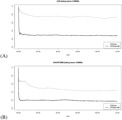
Classification Strategies. In this subsection, we compare the classification performance of VFDR using two different classification strategies. Assume that a rule covers a test example. The example might be classified either using the majority class of the training examples covered by the rule or using a naive Bayes directly derived from sufficient statistics stored in the rule. In this work, we designate as VFDR the algorithm that classify examples using the majority class strategy while VFDRNB designates the version that use naive Bayes classifiers. VFDRNB explores information about the distribution of attribute-values per class, P(xi|c). To have robust estimators of these probabilities, we require a minimum number of training examples covered by the rule 3 .
Figure 1 plots the evolution of the prequential error (Gama et al., 2009) for the LED and Waveform datasets. The VFDRNB exhibit much more powerful predicting capabilities than VFDR, especially in case of noisy data, as in LED dataset. Another observation is that VFDRNB exhibit very good performance at any-time, a relevant property in stream mining.
Since the behavior in the rest of the datasets is very similar to aforementioned cases we can conclude that the use of NB improves the predictive capabilities and therefore we proceed to compare and present the results of VFDRNB.
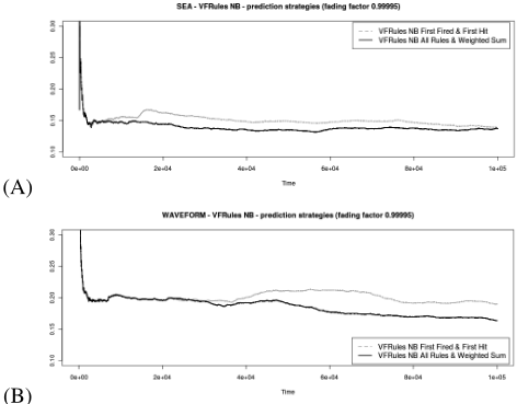
Ordered rules versus unordered rules. Classification rules offer a variety of different combinations of approaches for learning and predicting. In this section we focus on two strategies that we found potentially most interesting. It is a combination of learning (expanding) only one rule, the rule that first triggered, with predicting also according to a first hit strategy (VFDRo ). Obviously, for this approach it is necessary to use ordered rules. The second setting employs unordered rule set, where all the covering rules learn (expand) and the weighted sum of their predictions determines the final class prediction (VFDRu ).
3 This is a user defined parameter. We have used 50 examples in the experiments reported here.
| Unordered | Ordered |
|---|---|
| A = 1 ∧B = 1 → 1 C = 1 ∧D = 1 → 1 A = 0 ∧D = 0 → 0 B = 0 ∧D = 0 → 0 | 1. B = 0 ∧C = 0 → 0 2. A = 1 ∧B = 1 → 1 3. D = 0 → 0 4. B = 0 → 1 |
As we observed in the previous section, VFDRNB outperforms VFDR, therefore only this version is included in the following results. Both strategies have almost the same error rate in the simple nominal datasets, similar results in LED and SEA (Fig. 2(A)), and larger difference is only in Waveform, Fig. 2(B).
Ordered set focuses more on specializing one rule and as a result it often produces less rules than the other strategy. Although it is, indeed, a positive indicator it might not come without a price. Disjunctive can serve as a simple example. If we compare the two obtained rule sets in Tab. 1, we can notice the explicitly expressed rules that generates the dataset, whereas in the case of ordered rules one needs to consider the previous rules and remaining combinations, which might not be easy to interpret in more complex sets. Unordered rule sets are more modular, because they can be interpreted per si, while ordered rule sets must be interpreted in the context of previous rules.
Overall, the experimental results point out that unordered rule sets are more competitive than ordered rule sets in terms of error rate. In terms of number of rules, unordered rule sets tend to induce more rules than ordered rule sets.
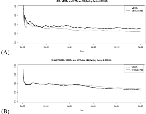
VFDRNB vs. VFDTc and C4.5rules. Having selected the most appropriate settings for VFDRNB, the last series of tests aim to disclose the differences between VFDRNB and its most similar rival VFDTc proposed by Gama et al. (2003), which also exploits NB classifier in the leaves to predict the class. In the most simple datasets Stagger and Disjunctive concept there is almost no difference between VFDTc and VFDRNB, both in terms of in error rate. Both quickly converge towards zero once the rules are learned (tree is grown). These are nice examples of the benefit of the representation provided by decision rules, which is much more convenient than a tree. Only five rules were induced, as opposed to seven leaves of decision tree in case of Disjunctive concept.
Figure 3(A) depicts the error-rate curves for VFDTc and VFDRNB in LED dataset. It reveals peaks in the error, especially during the early phase. They are caused by creation of new rules (leaves), consequential re-learning of NB and using the weak early classification abilities of very general rules. Nevertheless, learning process of this set requires lot of examples and even after observing all 100K examples the rules are not sufficient enough to make good prediction without NB, therefore the oscillations remain. In Waveform problem, Fig. 3(B), both combined classifiers achieve almost the same accuracy in prequential evaluation.
Table 2 summarizes the results from train and test experiments. C4.5rules failed to run with training sets of 106 examples (in LED, Waveform, and Hyperplane). The results reported here, corresponds to the maximum training set where we succeed: 200k. For numeric data sets, C4.5rules tends to generate very large theories, with excessive learning times and memory consumption. VFDRNB is very competitive against C4.5rules, using much less resources in terms of memory and learning times. The number of rules of VFDRo is as expected smaller than VFDRu in most of the cases with the exception of LED, which is presented in Table 3. Although the number of rules is quite large as opposed to VFDTc for numeric datasets, it could be reduced by carefully setting the necessary percentage of examples with vij value when computing best split evaluation.
Learning Times. VFDR was implemented in Java within the KNIME (Ad¨a and Berthold, 2010) data mining tool. For a fair comparison, we present the ratio of learning times of the proposed algorithms relative to KNIME implementation of VFDTc in the last columns of Table 3 for the set of experiments reported here. Values greater than one, means that rules are slower than VFDTc. We can observe than VFDRo has learning times of the same order of magnitude than VFDTc, while VFDRu is always slower than VFDRo . This is expected, because the number of rules learned by VFDRu increases faster than in VFDRo .
Bias-VarianceAnalysis. It is known that batch incremental algorithms are sensitive to the order of examples. Their biasvariance profile exhibit high variance. This is not the case of Hoeffding based algorithms that used to have low variance. This behavior is confirmed in the figures of the bias-variance decomposition of the error for VFDRoNB :
| loss | bias | var | |
|---|---|---|---|
| Waveform | 19.56 | 15.85 | 3.71 |
| Hyperplane | 21.32 | 17.99 | 3.33 |
5 Conclusions
In this paper we introduced a new decision rule classification approach for streaming data VFDR, which incrementally learns from incoming examples and expands rules over time. VFDR is a general purpose decision rule inducer, able to deal with multi-classes, nominal and continuous attributes. VFDR induces ordered and unordered rule sets. The experimental results point out that unordered rule sets, in comparison to ordered rule sets, are more competitive in terms of error rate, and more modular, in terms of interpretability, at the cost of inducing more rules. Moreover, the naive Bayes classification strategy used by rules strong improves the any-time characteristic of the classifier. The experimental evaluation show that VFDRNB is much more efficient than C4.5rules in terms of memory and learning times, and is competitive against VFDT, the state-of-the-art in streaming decision tree learning. The advantage is a more comprehensible and modular language to represent generalization, at least for tasks where understandability is relevant. We are now extending VFDR to deal with time-changing streams.
| Error rate % (variance) | |||||
|---|---|---|---|---|---|
| VFDRo | VFDRuNB | VFDRoNB | VFDTc | C4.5rules | |
| Disjunctive | 0 | 0 | 0 | 0 | 0 |
| Stagger | 0 | 0 | 0 | 0 | 0 |
| SEA | 23.7 | 12.9 | 13.2 | 11.9 | 10.5 |
| LED | 26.4 (0.05) | 25.6 (12.2) | 26.1 (0.04) | 26.0 (0.01) | 27.1 (0.34) |
| Hyperplane | 29.7 (14.63) | 24.2 (16.1) | 24.8 (12.7) | 23.1 (15.3) | 25.74 (15.6) |
| Waveform | 25.0 (1.66) | 16.9 (0.21) | 18.9 (0.05) | 15.74 (0.01) | 20.4 (0.18) |
| Size (number of rules/leaves) | Time (relative to VFDTc) | ||||||
|---|---|---|---|---|---|---|---|
| VFDRuNB | VFDRoNB | VFDTc | C4.5r | VFDRuNB | VFDRoNB | C4.5rules | |
| Disjunctive | 5 | 5 | 7 | 6 | 1 | 1 | 1 |
| Stagger | 5 | 3 | 4 | 5 | 1 | 1 | 1 |
| SEA | 85 | 50 | 36 | 77 | 2 | 2 | 10 |
| LED | 24 | 52 | 47 | 218 | 2.6 | 1 | 2.1 × 10³ |
| Hyperplane | 892 | 415 | 273 | 425 | 4.4 | 1.4 | 0.2 × 10³ |
| Waveform | 758 | 376 | 142 | 143 | 1.8 | 0.7 | 1.5 × 10⁵ |
Acknowledgements: This work was supported by FCT (PTDC/EIA-EIA/098355/2008) and Masaryk University.
@inproceedings{ijcai2011p213,
  title     = {Learning Decision Rules from Data Streams},
  author    = {Gama, Joao and Kosina, Petr},
  booktitle = {Proceedings of the Twenty-Second International Joint Conference on
               Artificial Intelligence, {IJCAI-11}},
  publisher = {AAAI Press/International Joint Conferences on Artificial Intelligence},
  editor    = {Toby Walsh},
  pages     = {1255--1259},
  year      = {2011},
  month     = {7},
  doi       = {10.5591/978-1-57735-516-8/IJCAI11-213},
  url       = {https://doi.org/10.5591/978-1-57735-516-8/IJCAI11-213},
}
TY - CPAPER TI - Learning Decision Rules from Data Streams AU - Gama, Joao AU - Kosina, Petr T2 - Proceedings of the Twenty-Second International Joint Conference on Artificial Intelligence, IJCAI-11 PB - AAAI Press/International Joint Conferences on Artificial Intelligence PY - 2011 SP - 1255 EP - 1259 DO - 10.5591/978-1-57735-516-8/IJCAI11-213 UR - https://doi.org/10.5591/978-1-57735-516-8/IJCAI11-213 ER -Copied
Machine-readable versions of this paper, for tools and AI agents:





