Approximation-Guided Evolutionary Multi-Objective Optimization

1 Introduction

Most real-world optimization problems are characterized by multiple objectives. As these objectives are often in conflict with each other, the goal of solving a multi-objective optimization (MOO) problem is to find a (not too large) set of compromise solutions. The Pareto front of a MOO problem consists of the function values representing the different trade-offs with respect to the given objective functions. Multi-objective optimization is assumed to be more (or at least as) difficult as single-objective optimization due to the task of computing several solutions. From a computational complexity point of view even simple single-objective problems on weighted graphs like shortest paths or minimum spanning trees become NP-hard when they encounter at least two weight functions [12]. In addition, the size of the Pareto front is often exponential for discrete problems and even infinite for continuous ones.

Due to the hardness of almost all interesting multiobjective problems, different heuristic approaches have been used to tackle them. Among these methods evolutionary algorithms are frequently used as they work at each time step with a set of solutions called population. The population of an evolutionary algorithm for a MOO is used to store desired trade-off solutions for the given problem.

As the size of the Pareto front is often very large, evolutionary algorithms and all other algorithms for MOO have to restrict themselves to a smaller set of solutions. This set of solutions should be a good approximation of the Pareto front. The main question is now how to define approximation. The literature (see e.g. [7]) on evolutionary multi-objective optimization (EMO) just states that the set of compromise solutions

• should be close to the true Pareto front,
• should cover the complete Pareto front, and
• should be uniformly distributed.

There are different evolutionary algorithms for multiobjective optimization such as NSGA-II [8], SPEA2 [19], or IBEA [18] which try to achieve these goals by preferring diverse sets of non-dominated solutions.

However, the above notion of approximation is not a formal definition. Having no formal definition of approximation makes it hard to evaluate and compare algorithms for MOO problems. Therefore, we think that it is necessary to use a formal definition of approximation in this context and evaluate algorithms with respect to this definition.

Different formal notions of approximation have been used to evaluate the quality of algorithms for multi-objective problems from a theoretical point of view. The most common ones are the multiplicative and additive approximation (see [6, 10, 17]). Laumanns et al. [16] have incorporated this notion of approximation in an evolutionary algorithm for MOO. However, this algorithm is mainly of theoretical interest as the desired approximation is determined by a parameter of the algorithm and is not improved over time. Another approach related to a formal notion of approximation is the popular hypervolume indicator [20] which measures the volume of the dominated portion of the objective space. Hypervolume-based algorithms such as MO-CMA-ES [15] or SMS-EMOA [2] are well-established for solving MOO problems. They do not use a formal notion of approximation but it has recently been shown that the worst-case approximation obtained by optimal hypervolume distributions is asymptotically equivalent to the best worst-case approximation achievable by all sets of the same size [4, 5]. The major drawback of the hypervolume approach is that it cannot be computed in time polynomial in the number of objectives unless P = NP [3].

In this paper, we introduce an efficient framework of an evolutionary algorithm for MOO that works with a formal notion of approximation and improves the approximation quality during its iterative process. The algorithm can be applied to a wide range of notions of approximation which are formally defined. As the algorithm does not have complete knowledge about the true Pareto front, it uses the best knowledge obtained so far during the optimization process.

The intuition for our algorithm is as follows. During the optimization process, the current best set of compromise solutions (usually called "population") gets closer and closer to the Pareto front. Similarly, the set of all non-dominated points seen so far in the objective space (we call this "archive") is getting closer to the Pareto front. Additionally, the archive is getting larger and larger and becoming an increasingly good approximation of the true Pareto front. Assuming that the archive approximates the Pareto front, we then measure the quality of the population by its approximation with respect to the archive. In our algorithm

• any set of feasible solutions constitutes an (potentially bad) approximation of the true Pareto front, and
• we optimize the approximation with respect to all solutions seen so far.

We show that this approach is highly successful in obtaining approximations according to the formal definition. Comparing our results to state of the art approaches such as NSGA-II, SPEA2, and hypervolume based algorithms, we show that our algorithm gives significantly better approximations fulfilling the formal definition.

The outline of this paper is as follows. We introduce some basic definitions in Section 2. The basic algorithm is presented in Section 3 and speed up techniques are discussed in Section 4. We report on our experimental results in Section 5 and finish with some conclusions.

2 Preliminaries

We consider minimization problems with d objective functions, where d ≥ 2 holds. Each objective function fi : S ↦→ R, 1 ≤ i ≤ d, maps from the considered search space S into the real values. In order to simplify the presentation we only work with the dominance relation on the objective space and mention that this relation transfers to the corresponding elements of S.

For two points x = (x1, . . . , xd) and y = (y1, . . . , yd), with x, y ∈ Rd we define the following dominance relation:

The typical notions of approximation used in theoretical computer science are multiplicative and additive approximation. We use the following definition

Definition 1. For finite sets S, T ⊂ Rd , the additive approximation of T with respect to S is defined as

This paper only regards additive approximation. However, our approach can be easily adapted to multiplicative approximation where in Definition 1 just the term si - ti has to be replaced by si/ti.

Algorithm 1: Measure approximation quality of a population

input : Archive A, Population P output: Indicator Sα(A, P )

1 S ← ∅; 2 foreach a ∈ A do 3 δ ← ∞; 4 foreach p ∈ P do 5 ρ ← -∞; 6 for i ← 1 to d do 7 ρ ← max{ρ, ai - pi}; 8 δ ← min{δ, ρ}; 9 S ←S ∪ {δ};

10 sort S decreasingly;

11 return S;

Algorithm 2: Insert point into archive

input : Archive A, Point p ∈ Rd

output: Archive consisting of the Pareto optimal points of A ∪ {p}

• 1 dominated ← false;
• 2 foreach a ∈ A do
• 3 if a ≺ p then delete a from A;
• 4 if a ⪰ p then dominated ← true;
• 5 if not dominated then add p to A;
• 6 return A;

Our aim is to minimize the additive approximation of the population P we output with respect to the archive A of all points seen so far, i.e., we want to minimize α(A, P ). The problem is that α(A, P ) is not sensitive to local changes of P . α(A, P ) only measures improvements of points which are currently worst approximated.

To get a sensitive indicator which can be used to guide the search, we consider instead the set {α({a}, P ) | a ∈ A} of all approximations of the points in A. We sort this set decreasingly and call the resulting sequence

The first entry α1 is again α(A, P ). Our new goal it then to minimize Sα(A, P ) lexicographically. Note that this is an augmentation of the order induced by α(A, P ): If we have α(A, P1) < α(A, P2) then we also have Sα(A, P1) <lex Sα(A, P2). Moreover, this indicator is locally sensitive. Algorithm 1 describes how to calculate it.

3 Simple Algorithm

Given the definition of Sα(A, P ), it is easy to come up with an algorithm which minimizes it lexicographically. Algorithm 3 presents such an algorithm. It maintains a population of μ individuals. In each generation, it generates λ new offspring. From the union of the old population and the offspring generation it iteratively removes the individual p for which Sα(A, P \ {p}) is lexicographically smallest. Every

1 Initialize population P with μ random individuals; 2 Set archive A←P; 3 foreach generation do 4 Initialize offspring population O ← ∅; 5 for j ← 1 to λ do 6 Select two random individuals from P; 7 Apply crossover and mutation; 8 Add new individual to O; 9 foreach p ∈ O do 10 Insert offspring p in archive A with Algorithm 2; 11 Add offsprings to population, i.e., P ←P ∪O; 12 while |P| > μ do 13 foreach p ∈ P do 14 Compute Sα(A, P \ {p}) with Algorithm 1; 15 Remove p from P for which Sα(A, P \ {p}) is lexicographically smallest;

new individual is added to the archive A such that the archive only contains non-dominating solutions. As described in Algorithm 2, this means that (i) a new offspring is only added if it is not dominated by another individual already in A and (ii) individuals in A which are dominated by a new individual are removed. Note that in contrast to many other algorithms (like Laumanns et al. [16] or all hypervolume-based algorithms), our new algorithms needs no meta-parameters.

We now give an upper bound for the runtime of Algorithm 2. One generation consists of producing and processing λ offspring. The main part of the runtime is needed for the O(λ(μ + λ)) computations of Sα(A, P \ {p}), each costing O(d |A| (μ + λ) + |A| log |A|). Hence, we get a runtime of O(λ(μ + λ) |A| (d (μ + λ) + log |A|)) for generating an offspring of λ points. This means for N function evaluations, that is, N generated points overall, we get a total runtime of

This algorithm works well for small population and offspring sizes μ + λ, but for e.g. μ + λ = 100, it becomes very slow due to the (μ + λ)2 factor.

4 Fast Algorithm

We now show how to speed-up our approach. Let us first assume that the approximations α({a}, {p}) are distinct for all a ∈ A and p ∈ P. For all a ∈ A we denote the point p ∈ P that approximates it best by p1(a) and the second best by p2(a). The respective approximations we denote by αi(a) := α({a}, {pi(a)}) for i ∈ {1, 2}. Now, let p ̸= q ∈ P and consider Sp := Sα(A, P \ {p}) and Sq := Sα(A, P \ {q}). Significant for the comparison of the two are only the positions a ∈ A where Sp or Sq differ from S := Sα(A, P ). This is the case for all positions in B := {a ∈ A | p1(a) ∈ {p, q}}. If we delete p from P , then the worst approximation of one of the a ∈ B is the maximum of max{α2(a) | p1(a) = p} and max{α1(a) | p1(a) = q}. Now observe that if

1 1-1 See lines 1-11 of Algorithm 3 12 foreach a ∈ A do 13 p1(a) ← argminp∈P α({a}, {p}); 14 p2(a) ← argminp1(a)̸=p∈P α({a}, {p}); 15 α1(a) ← minp∈P α({a}, {p}); 16 α2(a) ← minp1(a)̸=p∈P α({a}, {p}); 17 foreach p ∈ P do 18 β(p) ←maxa∈A{α2(a) | p1(a) = p}; 19 while |P| > μ do 20 Remove p∗ from P with β(p) maximal; 21 foreach a ∈ A with p1(a) = p∗ do 22 Compute p1(a), p2(a), α1(a), α2(a) as done above in lines 13-16; 23 β(p1(a)) ← max{β(p1(a)), α2(a)};

is smaller than the respective β(q), then also the larger term above is smaller, as max{α1(a) | p1(a) = q} < max{α2(a) | p1(a) = q}. Hence, we end up with the fact that we only have to compare β(p) and throw out the point p with β(p) maximal (see Algorithm 4).

Recall that we assumed that all approximations α({a}, {p}) with a ∈ A, p ∈ P are distinct. If this does not hold, we can simply change the indicator Sα(A, P ) slightly and insert symmetry breaking terms a · ε, where ε > 0 is an infinitesimal small number. This means that we treat equal approximations as not being equal and hence in some arbitrary order.

We now give an upper bound for the runtime of Algorithm 4. For one generation, i.e., for producing and processing λ offspring, the algorithm needs a runtime of O(d (μ + λ) |A|) for computing the values p1(a), p2(a), α1(a), α2(a) and β(p) initially. Then we repeat λ times: We delete the point p∗ ∈ P with β(p) maximal in O(μ + λ), after which we have to recompute the values p1(a), p2(a), α1(a), α2(a), but only for a ∈ A with p1(a) = p∗ . Observe that we can store a list of these a's during the initial computation and keep these lists up to date with no increase of the asymptotic runtime. Also note that we would expect to find O(|A|/|P|) points with p1(a) = p∗ , while in the worst case there may be up to O(|A|) such points. Summing up, we get a heuristic runtime for one generation of O(d (μ + λ) |A|+ λ((μ + λ) + d|P | · |A|/|P |)) which simplifies to O(d(μ + λ)|A|) as |A| ≥ μ + λ. In the worst case we replace O(|A|/|P |) by O(|A|) and get a runtime for one generation of O(dλ(μ + λ)|A|). For N fitness evaluations we, therefore, get a runtime of O(d(1+ μ/λ)|A|N ) heuristically, and O(d(μ + λ)|A|N ) in the worst case. Note that |A| ≤ N. For any λ = O(μ), e.g. λ = 1 or λ = μ, this can be simplified to O(dμ|A|N ) in both cases, while for λ = Ω(μ), e.g. λ = μ, we get a reduced heuristic runtime of O(d|A|N ).

5 Experimental Study

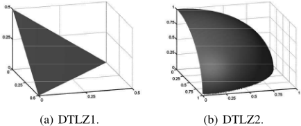
The fast (μ + λ)-version of our algorithm was implemented in the jMetal framework [11]. The code is available upon request. We compared the performance of our AGE algorithm to the established MOO algorithms IBEA [18], NSGA-II [8], SMS-EMOA [13], and SPEA2 [19] on the DTLZ benchmark family [9]. We used the functions DTLZ 1-4, each with 30 function variables and between 2 to 20 objective values/dimensions. Figure 3 shows the Pareto fronts of DTLZ1 and DTLZ2 for three objectives. The fronts of DTLZ3 and DTLZ4 are equivalent to DTLZ2; they only differ in the mapping from the search space to the objective space. We limit the calculations of the algorithms to a maximum of 100,000 fitness evaluations and a maximum computation time of four hours per run. Note that the time restriction had to be used as the runtime of some algorithms increases exponentially with respect to the size of the objective space.

The further parameter setup of the algorithms was as follows. Parents were selected through a binary tournament, in which we selected the individual out of two randomly drawn ones with the better approximation of the archive. As variation operators, the polynomial mutation and the simulated binary crossover [1] were applied, which are both used widely in MOO algorithms [8, 14, 19]. The distribution parameters associated with the operators were ηm = 20.0 and ηc = 20.0. The crossover operator is biased towards the creation of offspring that are close to the parents, and was applied with pc = 0.9. The mutation operator has a specialized explorative effect for MOO problems, and was applied with pm = 1/(number of variables).

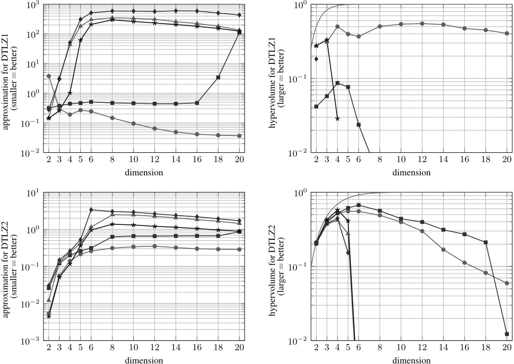
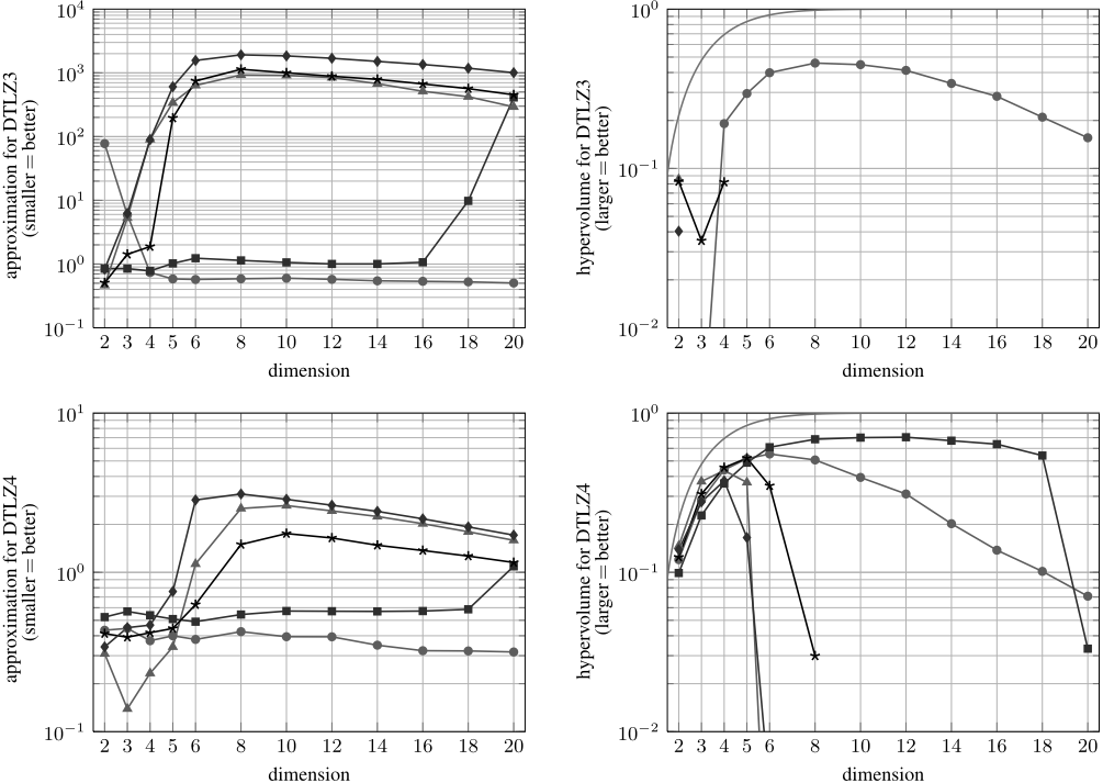
Figures 1 and 2 present our results for population size μ = 100 and λ = 100, averaged over 100 independent runs. We performed the same experiments also for μ ∈ {25, 50} and observed similar behaviors. We assess the algorithms using

the following measures:

• Approximation: We approximate the achieved additive approximation of the known Pareto fronts by first drawing one million points of the front uniformly at random and then computing the approximation which the final population achieved for this set with Algorithm 1.
• The hypervolume [20] is a popular performance measure which measures the volume of the dominated portion of the objective space relative to a reference point r. For DTLZ1 we choose r = 0.5d , otherwise r = 1d . We approximate the achieved hypervolume with an FPRAS [3] which has a relative error of more than 2% with probability less than 1/1000. The volumes shown for DTLZ1 are normalized by the factor 2d .

As it is very hard to determine the minimum approximation ratio achievable or the maximum hypervolume achievable for all populations of a fixed size μ, we only plot the theoretical maximum hypervolume for μ → ∞. For this, a simple geometric calculation gives a maximum (rescaled) hypervolume of 1 - 1/d! for DTLZ1 and a maximum hypervolume of 1 - 2-d πd/2/(d/2)! for DTLZ2 (with n! := Γ(n + 1)).

For all test functions, our new algorithm AGE ( ) achieves the best approximation among the competing algorithms for dimensions d > 5. We first discuss DTLZ1 and DTLZ3 who are known to be hard to analyze as they contain a very large number of local Pareto-optimal fronts [9]. For both functions, we achieve the best approximation among all tested algorithms for d > 3. Remarkably, all other algorithms (besides IBEA ( )) are unable to find the front at all for these instances. This results in extremely large approximations and zero hypervolumes. The reason for IBEAs decreasing behaviour for very large dimension (d ≥ 18) is that it was stopped after four hours and it could not perform 100′ 000 iterations. The same holds already for much smaller dimensions in the case of SMS-EMOA ( ), which uses an exponential-time algorithm to internally determine the hypervolume. It did not finish a single generation for d ≥ 8 and only performed around 5′ 000 iterations within four hours for d = 5. This implies that the higher-dimensional approximations plotted for SMS-EMOA ( ) actually show the approximation of the random initial population. Interestingly, the approximations achieved by NSGA-II ( ) and SPEA2 ( ) are even worse as they are tuned for lowdimensional problems and move their population too far out to the boundaries for high dimensions. Our algorithm ( ) and also NSGA-II ( ) and SPEA2 ( ) always finished in less than four hours.

The plots of DTLZ2 and DTLZ4 reveal other properties. Here, an approximation of the front seems generally much easier. For small dimensions (d = 2, 3, 4), all algorithms find acceptable solutions. However, for larger dimensions again SMS-EMOA ( ), NSGA-II ( ), and SPEA2 ( ) fail for the said reasons. In these cases, our algorithm ( ) still achieves the best approximation, but for 4 ≤ d ≤ 18 (DTLZ2) and 6 ≤ d ≤ 18 (DTLZ4), the solutions found by IBEA ( ) (which uses the hypervolume as an indicator) have a larger hypervolume. The hypervolume of IBEA is only worse for d = 20 because it could only perform a few hundred iterations within the four hour time limit.

6 Conclusions

Evolutionary algorithms are frequently used to solve multiobjective optimization problems. Often, it is very hard to formally define the optimization that current state-of-the-art approach work with. We have presented a new evolutionary multi-objective algorithm that works with a formal notion of approximation. The framework of our algorithm allows to work with various formal notions of approximations. Our experimental results show that given a fixed time budget it outperforms current state-of-the-art approaches in terms of the desired additive approximation as well as the covered hypervolume on standard benchmark functions. This holds, in particular, for problems with many objectives, which most other algorithms have difficulties dealing with.