
The Multi-Inter-Distance Constraint
Proceedings of the Twenty-Second International Joint Conference on Artificial Intelligence. Pages 629-633.
https://doi.org/10.5591/978-1-57735-516-8/IJCAI11-112
© 2011 International Joint Conferences on Artificial Intelligence
Abstract
We introduce the MULTI-INTER-DISTANCE constraint that ensures no more than m variables are assigned to values lying in a window of p consecutive values. This constraint is useful for modeling scheduling problems where tasks of processing time p compete for m identical resources. We present a propagator that achieves bounds consistency in cubic time. Experiments show that this new constraint offers a much stronger filtering than an edge-finder and that it allows to solve larger instances of the runway scheduling problem.
- [Artiouchine & Baptiste, 2005] Artiouchine, K., and Bap- tiste, P. 2005. Inter-distance constraint: An extension of the all-different constraint for scheduling equal length jobs. In Proc. of the 11th Int. Conf. on Principles and Practice of Constraint Programming, 62-76.
- [Artiouchine, Baptiste, & Dürr, 2004] Artiouchine, K.; Bap- tiste, P.; and Dürr, C. 2004. Runway scheduling with hold- ing loop. In Proc. of 2nd Int. Workshop on Discrete Opti- mization Methods in Production and Logistics, 96-101.
- [Cormen et al., 2001] Cormen, T. H.; Stein, C.; Rivest, R. L.; and Leiserson, C. E. 2001. Introduction to Algorithms. McGraw-Hill Higher Education, 2nd edition.
- [Dürr & Hurand, 2009] Dürr, C., and Hurand, M. 2009. Finding total unimodularity in optimization problems solved by linear programs. Algorithmica. DOI 10.1007/s00453-009-9310-7. DOI
- [Leconte, 1996] Leconte, M. 1996. A bounds-based reduc- tion scheme for constraints of difference. In Proc. of the Constraint Int. Workshop on Constraint-Based Reasoning, 19-28.
- [López-Ortiz & Quimper, 2011] López-Ortiz, A., and Quim- per, C.-G. 2011. A fast algorithm for multi-machine scheduling problems with jobs of equal processing times. In In 28th Int. Symp. on Theoretical Aspects of Computer Science (to appear in STACS'11).
- [Mercier & Hentenryck, 2008] Mercier, L., and Hentenryck, P. V. 2008. Edge finding for cumulative scheduling. IN- FORMS Journal on Computing 20(1):143-153.
- [Quimper, López-Ortiz, & Pesant, 2006] Quimper, C.-G.; López-Ortiz, A.; and Pesant, G. 2006. A quadratic propagator for the inter-distance constraint. In Proc. of the 21st Nat. Conf. on Artificial Intelligence (AAAI 06), 123-128.
- [Régin, 1994] Régin, J.-C. 1994. A filtering algorithm for constraints of difference in CSPs. In Proc. of the 11th National Conference on Artificiel Intelligence (AAAI-94), 362-367.
- [Régin, 1996] Régin, J.-C. 1996. Generalized arc consis- tency for global cardinality constraint. In Proc. of the 8th Annual Conference on Innovative Applications of Artificial Intelligence, 209-215.
- [Vilím, Barták, & Cepek, 2004] Vilím, P.; Barták, R.; and Cepek, O. 2004. Unary resource constraint with optional activities. In Proc. of the 10th Int. Conference on Princi- ples and Practice of Constraint Programming, 62-76.
- [Vilím, 2009] Vilím, P. 2009. Edge finding filtering algo- rithm for discrete cumulative resources in o(kn log n). In Proc. of the 15th Int. Conference on Principles and Prac- tice of Constraint Programming, 802-816.
References were extracted automatically from the PDF and may contain errors.
Full text extracted automatically from the PDF; figures, tables and equations may differ. The PDF is the version of record.
1 Introduction
Constraint solvers offer many ways to model scheduling problems. The constraint ALL-DIFFERENT [R´egin, 1994] ensures that at most one task starts at a given time. When there are m resources, the GCC [R´egin, 1996] limits the number of tasks starting at a given time to m. These two constraints are useful when tasks have a unit processing time. When processing times are greater than one unit, the INTER-DISTANCE [Artiouchine & Baptiste, 2005; Quimper, L´opez-Ortiz, & Pesant, 2006] constraint makes sure that the starting times are at least p units of time apart. When processing times differ for each task, the CUMULATIVE [Mercier & Hentenryck, 2008; Vil´ım, 2009] constraint allows to model this situation. All constraints, except the CUMULATIVE constraint, offer a complete filtering of the release times and deadlines of the task in polynomial time. This filtering is NP-Hard for the CUMULATIVE constraint. However, there exists no filtering algorithm that prunes the release times and deadlines when the processing time of each task is p and when there are m > 1 resources. We introduce the MULTI-INTER-DISTANCE constraint and its first filtering algorithm achieving bounds consistency. This constraint complements the offering of constraint solvers. We show that this constraint is very efficient to solve problems such as the runway scheduling problem.
2 The MULTI-INTER-DISTANCE Constraint
The MULTI-INTER-DISTANCE constraint limits the number of variables assigned in a window of p consecutive values to m. Definition 1 formally presents the constraint.
Definition 1 MULTI-INTER-DISTANCE([X1, . . . ,Xn],m, p) is satisfied if and only if at most m variables Xi are assigned to a value in any window of p consecutive values. More formally, we have the following logical identity.
The MULTI-INTER-DISTANCE is a generalization of well known constraints. When p = 1 and m = 1, the MULTI-INTER-DISTANCE constraint specializes into an ALL-DIFFERENT constraint. When p = 1 and m > 1, the MULTI-INTER-DISTANCE encodes a GCC where each value can be assigned to at most m variables. Finally, with m = 1 and p > 1, the MULTI-INTER-DISTANCE becomes an INTER-DISTANCE constraint. On the other hand, the MULTI-INTER-DISTANCE constraint is a specialization of the CUMULATIVE constraint. Each variable can be seen as the starting time of a task that consumes one unit of resource during a period of time p where the cumulative capacity of the resources is m.
Two results emerge from these relations among the constraints. Since it is NP-Hard to enforce domain consistency on the INTER-DISTANCE constraint [Artiouchine, Baptiste, & D¨urr, 2004], it is necessarily NP-Hard to enforce domain consistency on the MULTI-INTER-DISTANCE. Because the edge-finder [Mercier & Hentenryck, 2008; Vil´ım, 2009] does not enforce bounds consistency on the INTER-DISTANCE [Artiouchine & Baptiste, 2005], it does not enforce bounds consistency on the MULTI-INTER-DISTANCE either.
We show how to detect feasibility of the MULTI-INTER-DISTANCE constraint in quadratic time. We then show how bounds consistency can be enforced in cubic time.
3 General Background
We consider constraint satisfaction problems where variables are assigned to integer values. The domain of a variable Xi is denoted dom(Xi). We assume that the domain of a variable dom(Xi) = [li, ui) is a semi-open interval where li and ui are called the lower bound and upper bound of the domain. The value of the variable Xi must be greater than or equal to li and must be strictly smaller than ui.
An interval support for a value v ∈ dom(Xi) with respect to a constraint C(X1, . . . ,Xn) is a tuple t satisfying three conditions for j ∈ 1..n: 1) lj ≤ t[j] < uj, 2) t[i] = v and 3) the tuple (t[1], . . . , t[n]) satisfies the constraint C. A constraint is bounds consistent if li and ui - 1 have an interval support for all i = 1..n. Enforcing bounds consistency on a constraint consists of increasing the lower bounds and decreasing the upper bounds of the domains until all bounds have an interval support. Example 1 shows the result of enforcing bounds consistency on the MULTI-INTER-DISTANCE constraint.
Example 1 We consider the constraint MULTI-INTER-DISTANCE([X1, X2, X3, X4, X5], m, p) with m = 2, p = 3, and the following domains.
The domains are semi-open intervals which implies that the value 1 belongs to the domain of X1 but the value 9 does not belong to the domain of X1.
Enforcing bounds consistency on the MULTI-INTER-DISTANCE shrinks the domains as follows.
4 Testing for Satisfaction in Polynomial Time
The MULTI-INTER-DISTANCE has a strong connection to scheduling problems. Consider the constraint MULTI-INTER-DISTANCE([X1, . . . ,Xn],m, p) where the domain of the variable Xi is the semi-open interval [li, ui). The variable Xi can be considered as the starting time of a task whose processing time is p, whose release time is li, and whose deadline is ui + p - 1. A total of m identical resources execute the tasks concurrently without preemption. The MULTI-INTER-DISTANCE constraint is satisfiable if and only if there exists a schedule.
This scheduling problem can be solved in polynomial time. The best algorithm [L´opez-Ortiz & Quimper, 2011] so far has a worst-case time complexity of O(n2 min(1, pm )). The algorithm finds a valid schedule by computing a shortest path in a scheduling graph [D¨urr & Hurand, 2009]. This section provides a description of this graph and its properties. The scheduling graph is the key concept on which the filtering algorithm is based.
Let lmin = mini li and umax = maxi ui be the smallest lower bound and the greatest upper bound of a variable domain. The scheduling graph G has a node v for every integer lmin ≤ v ≤ umax. There is a forward edge of weight m from node v to node v + p for all lmin ≤ v ≤ umax - p. For every pair of lower bound and upper bound li < uj, there is a backward edge (uj, li) of weight -|{k | li ≤ lk ∧ uk ≤ uj}|. The absolute value of the weight of the backward edge (uj, li) is the number of variables whose domain is contained in the interval [li, uj). A backward edge can have a null weight. There is a null edge from any node v + 1 to node v of weight 0 for all v ∈ [lmin, umax). Finally,
Table 1: The weight matrix of the scheduling graph of Example 1. Empty entries indicate the lack of an edge between nodes α and β.
.
there is an edge (lmin, umax) of weight n where n is the arity of the MULTI-INTER-DISTANCE constraint.
Table 1 shows the weight matrix of the scheduling graph of the problem depicted in Example 1. The scheduling graph has important properties that we state here. Theorem 1 provides the sufficient and necessary condition to test whether the scheduling problem has a solution.
Theorem 1 ([L´opez-Ortiz &Quimper, 2011]) The scheduling problem has a solution if and only if the scheduling graph has no negative cycles.
Theorem 2 ([L´opez-Ortiz &Quimper, 2011]) Testing whether there is a negative cycle in the scheduling graph can be done in O(n2 min(1, pm )) time.
Theorems 1 and 2 allow to test the satisfiability of the constraint in quadratic time. In the next sections, we reuse this result to design an efficient filtering algorithm.
5 Conditions toMaintain Bounds Consistency
Our filtering algorithm detects forbidden sets of values that cannot be assigned to a set of variables. For the ALLDIFFERENT constraint, these sets are called Hall intervals [Leconte, 1996]. For the MULTI-INTER-DISTANCE, we call them forbidden regions. We present lemmas that detect these forbidden regions.
To test whether an interval [a, b) is a forbidden region to which a variable Xi is subject, one can modify the domain of Xi to be [a, b) and test the satisfiability of the problem. If the scheduling graph of the transformed problem has a negative cycle, then [a, b) is a forbidden region for Xi.
We define the altered scheduling graph Gvi like the scheduling graph with one exception, we alter the upper bound of the domain of Xi such that the new domain becomes [li, v). If Gvi has a negative cycle, the constraint has no solution and we conclude that Xi ≥ v. Table 1 gives the weight matrix of the graph G. Decrementing bold entries by one results in the altered scheduling graph G53 . In the graph G53 , the edges (5, 2) and(2, 5) form a cycle of weight -1 which proves that X3 ≥ 5. The following theorem shows how a forbidden region for one variable can also be a forbidden region for another variable.
Theorem 3 Let Xi and Xj be two variables whose domains satisfy ui ≤ uj. If the values in [li, v) have no interval support in dom(Xi), then they do not have an interval support in dom(Xj) either.
Proof: We prove the contraposition: if there exists a value a ∈ [li, v) that has an interval support in the domain of Xj then there exists a value b ∈ [li, v) that has an interval support in the domain of Xi. Suppose there exists an interval support t such that t[j] ∈ [li, v), we want to prove that there exists an interval support t′ such that t′ [i] ∈ [li, v). Two cases can occur. If t[i] ≤ t[j] then the inequalities li ≤ t[i] ≤ t[j] < v hold and t[i] ∈ [li, v). The theorem holds with t′ = t. However, if t[i] > t[j] the inequalities lj ≤ t[j] < t[i] ≤ ui ≤ uj hold. We can permute the values t[i] and t[j] to obtain the support t′ . We have t′ [i] = t[j] ∈ [li, v) and t′ [j] = t[i] ∈ [lj, uj) hence t′ is a valid support. ✷
In Example 1, the graph G53 has a negative cycle which proves that [4, 5) is a forbidden region for X3. Theorem 3 also makes [4, 5) a forbidden region for the variable X4.
The distance matrix DG of a graph G is a square matrix such that DG[a, b] is the shortest distance between node a and node b in graph G. This matrix exists only if there are no negative cycles in the graph G. When comparing the scheduling graph G of Example 1 and the altered scheduling graph G53 , one sees that the weights of a subset of the edges are decremented by one. This can only lead to shorter paths in G53 than in G. Lemma 1 captures this property.
Lemma 1 Let G be the scheduling graph of a problem where the domains are given by the intervals [li, ui) for 1 ≤ i ≤ n. Let G′ be the scheduling graph of the same problem except that the domain of Xi is changed to [l′i , u′i ) where li ≤ l′i < u′i ≤ ui holds. Thus DG[a, b] ≥ DG′ [a, b] holds for all pairs of nodes (a, b).
Proof: The weight of a backward edge (uj, lk) is minus the number of variable domains contained in the interval [lk, uj). If the domain of a variable is shrunk, the weight of the backward edges can be decremented by one or remain unchanged. These changes to the scheduling graph can only favor shorter paths.
However, the backward edges outgoing from ui or incoming to li may not exist in G′ as ui and li may not be domain bounds after shrinking the domain of Xi. Let (uf , le) be a backward edge in G such that f = i ∨ e = i. We prove that the edge (uf , le) in G can be replaced by an equivalent path in G′i . Let u′f = max({uk | uk ≤ uf ∧ k ̸= i} ∪ {u′i }) and let l′e = min({lk ≥ le ∧ k ̸= i} ∪ {l′i}). The weight of the backward edge (u′f , l′e ) in G′i is the same as the weight of the backward edge (uf , le) in G. Moreover, we have le ≤ l′e and u′f ≤ uf . Any path in G passing by the edge (uf , le) can be replaced by a sequence of null edges from uf to u′f , then passing by the edge (u′f , l′e ), and completing with a sequence of null edges from l′e to le. This path in G′i has the same weight as the edge (uf , le) in G. ✷
Let U = {ui | i ∈ 1..n} be the set of the domain upper bounds and let u∗ = min{u ∈ U | u > li} be the smallest upper bound that does not make the interval [li, u∗ ) empty. The altered scheduling graph Gu∗ i gives information about how the lower bound of Xi can be filtered. If Gu∗ i has a negative cycle, then Xi ≥ u∗ and the lower bound li can be safely increased to u∗ . If Gu∗ i has no negative cycle, then Theorem 4 and Theorem 5 indicates how to prune the lower bound of variable Xi.
Theorem 4 Let Xi be a variable subject to a MULTI-INTER-DISTANCE constraint. Let u∗ be the smallest upper bound that is greater than li, and let Gu∗ i be its associated altered scheduling graph. Suppose this graph has no negative cycle. Let t be the largest value such that the distance DGu∗ i [li, t] is null. Values smaller than t in the domain of Xi have no interval support.
Proof: SinceGu∗ i has no negative cycles, there exists at least one solution with Xi ∈ [li, u∗ ) where u∗ = min{uk | uk > li}. Let t be the largest value for which the shortest distance in Gu∗ i from li to t is null. We prove by contradiction that t < u∗ . Suppose t ≥ u∗ . The weight of the edge (u∗ , li) is at most -1 since it fully contains the altered domain of Xi. Contradictorily, there is a negative cycle in Gu∗ i starting from li, going to t through a path of weight zero (by definition of t), passing by the null edges (t, t-1), (t-1, t-2), . . . , (u∗ + 1, u∗ ) with weight zero, and then going back to li using the edge (u∗ , li) with weight at most -1. Therefore, t < u∗ .
Knowing that t < u∗ , we construct the altered scheduling graph Gti using the original variable domains except for Xi for which we use the domain dom(Xi) = [li, t). The edge (t, li) has a negative weight since the interval [li, t) contains the domain of Xi. The distance from li to t is null in Gu∗ i and, by Lemma 1, no greater than 0 in Gti . Therefore, there is a negative cycle in Gti passing by the edge (t, li) which implies that no values in [li, t) have an interval support in dom(Xi). ✷
To illustrate Theorem 4, consider the variable X1 in Example 1. The smallest upper bound that is greater than the lower bound 7 is u∗ = 9. The altered scheduling graph G91 is identical to the scheduling graph G. The path (7, 2), (2, 5), (5, 8) has a null weight in G91 . By Theorem 4, there is no valid assignment with X1 < 8.
Theorem 4 shows there is no interval support Xi ∈ [li, t). Theorem 5 shows that there is an interval support for Xi = t.
Theorem 5 Let Xi be a variable subject to a MULTI-INTER-DISTANCE constraint. Let u∗ be the smallest upper bound that is greater than li, and let Gu∗ i be its associated altered scheduling graph. Suppose this graph has no negative cycle. Let t be the largest value such that the distance DGu∗ i [li, t] is null. The value t has an interval support in the domain of Xi.
Proof: We construct the scheduling graph Gt+1 i using the original variable domains except for Xi for which we use the domain [li, t + 1). If one proves that Gt+1 i has no negative cycle, then one proves there is a solution with Xi ∈ [li, t+1).
Theorem 4 ensures that Xi ≥ t leaving Xi = t as the unique valid assignment for the variable Xi. The graph Gt+1 i has no negative cycles when t + 1 = u∗ . Indeed, in that specific case, the graphs Gt+1 i and Gu∗ i are by construction identical. From the proof of Theorem 4, we know that t ≤ u∗ . We therefore need to prove that Gt+1 i has no negative cycleswhen t + 1 < u∗ .
Let uq be the greatest upper bound that is strictly smaller than u∗ . By construction, there is no upper bounds greater than li and smaller than u∗ , thus uq < li. The null edges form a path from li to uq which implies DGt+1 i [li, uq] ≤ 0. Consider any lower bound lp that is smaller than or equal to li. The domain dom(Xi) = [li, t + 1) is the only one that is not contained in the interval [lp, uq) but is contained in the interval [lp, t + 1), thus -w(uq, lp) = -w(t + 1, lp) - 1.
The graphs Gu∗ i and Gt+1 i are very similar. They only differ by the additions of backward edges (t+1, lq) for all lower bound lq ≤ li. It is therefore sufficient to prove that any cycle passing by these edges has a non-negative weight.
Since the addition of the edges leaving t + 1 does not affect the paths leading to t + 1, we have DGt+1 i [li, t + 1] = DGu∗ i [li, t + 1]. By the definition of t, we obtain 0 < DGu∗ i [li, t + 1] = DGt+1 i [li, t + 1]. The consequence of this inequality is that any path going from li to t+1 has a positive weight and in particular, a path going from li to t +1 passing by the edge (uq, lp) has positive weight.
By substituting -w(uq, lp) = -w(t + 1, lp) - 1 and DGt+1 i [li, uq] ≤ 0 in (1) we prove that all cycles passing by the edge (t + 1, lp) are non-negative.
✷
In Example 1, the path (7, 2), (2, 5), (5, 8) in G91 has a null weight which certifies that there exists an interval support for 8 in the domain of X1. This interval support is t = [8, 2, 5, 6, 3].
6 A Filtering AlgorithmAchieving Bounds Consistency
The filtering algorithm for the MULTI-INTER-DISTANCE is a direct application of Theorem 3, Theorem 4, and Theorem 5. The algorithm on Figure 1 processes the variables in nondecreasing order of domain upper bounds. When processing Xi, the algorithm updates the lower bound li according to previously discovered fobidden regions. Then it computes the value u∗ that is the smallest domain upper bound greater than li. Based on this value, the algorithm tests whether the scheduling graph Gu∗ i has a negative cycle. If so, the algorithm stores in the data structure F the newly detected forbidden region [li, u∗ ). Because the algorithm processes variables in non-decreasing order of upper bounds, Theorem 3 ensures that the interval [li, u∗ ) is a forbidden region for all unprocessed variables. On its next iteration, the lower bound li is increased to avoid all forbidden regions, including the newly discovered one. This process continues until the scheduling graph Gu∗ i contains no negative cycles.
When the scheduling graph Gu∗ i contains no negative cycles, Theorem 4 and Theorem 5 apply. The algorithm computes the shortest path from node li to all the other nodes and finds the node t which is the largest one whose distance from node li is null. From Theorem 4, we know that values smaller than t have no interval support in the domain of the current variable. The algorithm removes them from the domain by increasing the value of li. Finally, Theorem 5 guarantees that the lower bound of each variable domain has an interval support upon completion of the algorithm.
Algorithm 1: PruneLowerBounds([X1, . . . ,Xn])
Sort the variables such that ui ≤ ui+1 U ← {u1, . . . , un} F ← ∅ for i ∈ 1..n do repeat li ← min([li, ui) \ F ) u∗ ← min((li, ui] ∩ U) Let Gu∗ i be the altered scheduling graph with dom(Xi) = [li, u∗ ) Compute the shortest distances DGu∗ i [li, t] from node li to all the other nodes t if there is a negative cycle in Gu∗ i then F ← F ∪ [li, u∗ ) until there is no negative cycles in Gu∗ i li ←max({t | DGu∗ i [li, t] = 0})Computing the single-source shortest path in the scheduling graph should be done with care. Indeed, the scheduling graph has as many nodes as the number of values in the domains. These domains can be very large especially in scheduling problems where domains represent time intervals. [L´opez-Ortiz & Quimper, 2011] showed how to compute the shortest path from the right-most node to all the other nodes in O(n2 min(1, pm )) steps which is strongly polynomial and invariant in the cardinality of the variable domains. The algorithm is an adaptation of the Bellman-Ford algorithm [Cormen et al., 2001] which initializes a distance vector that keeps track of the distances from the node li to all the other nodes. Since the right-most node can reach all the other nodes via the null edges, the distance vector is initialized to zero and as new paths are explored, the distance vector is updated with smaller values. To compute the shortest path from li to all the other nodes, the distance vector should be initialized to zero for all the nodes smaller than or equal to li and n for all the nodes that are greater than li. Indeed, any node t can be reached by going to lmin through the null edges, then going to umax using the edge (lmin, umax), and finally using the null edges to go to t. This simple adaptation to the shortest path algorithm is sufficient to compute the shortest path from the source node li to all the other nodes or to detect a negative cycle. The running time complexity remains O(n2 min(1, pm )).
The computation of shortest paths dominates the algorithms's complexity.
Lemma 2 The algorithm PruneLowerBounds performs at least n and at most 3n - 1 shortest path computations where n is the number of variables.
Proof: Computing the shortest path of an altered scheduling graph leads to two possible outcomes: the graph has negative cycles or it does not. If the graph has no negative cycles, the repeat loop terminates. This occurs exactly n times, once for each variable. If the graph has negative cycles, the algorithm loops and create the forbidden region [li, u∗ ). The value u∗ is a domain upper bound. Each time a new forbidden region is created, one of two events can occur: 1) a domain upper bound becomes for the first time the open upper bound of a forbidden region 2) a domain upper bound gets included in forbidden region. These two events can occur only once for each upper bound at the exception of the largest upper bound umax for which only the first event can occur. Therefore, the algorithm creates at most 2n - 1 forbidden regions and performs at most 3n - 1 shortest path computations. ✷
The shortest path problem is solved in O(n2 min(1, pm )) steps when using the algorithm of [L´opez-Ortiz & Quimper, 2011] and modifying the initial state of the distance vector as described above. The total running time complexity of the filtering algorithm is therefore O(n3 min(1, pm )) which is never more than O(n3 ).
Pruning the upper bounds can be done by pruning the lower bounds in a symmetric problem where dom(X′ i ) = [-ui, -li). When pruning the lower bounds, the value -ui is increased which is equivalent to decrease the upper bound ui in the original problem.
7 Experiments
We experiment the MULTI-INTER-DISTANCE on the runway scheduling problem as presented in [Artiouchine & Baptiste, 2005]. This problem consists of determining the order in which n airplanes should land on a runway. We consider an airport with m runways allowing simultaneous landings. Each airplane labeled from 1 to n has multiple disjoint time windows [ai1 , bi1 ], . . . , [aiki , biki ] in which it is in position to land. The goal is to make each airplane land within one of its time windows while maximizing the time gap p between each landing on a same runway.
We model the problem with two variables per airplane. The variable Si defines at what time the airplane i lands. The variable Wi ∈ [1, ki] defines in which time window the airplane i lands. The two variables are connected with the constraints Wi ≤ w ⇐⇒ Si ≤ biw and Wi ≥ w ⇐⇒ Si ≥ aiw . Finally, there is a MULTI-INTER-DISTANCE posted on the vector of variables S with fixed parameter p and m. We solve the problem for p = 1, 2, 4, 8, . . . until the problem becomes infeasible. We then perform a binary search between the largest p for which there exists a solution and the smallest p for which we detect infeasibility. We branch on the variables Wi followed by the variables Si.
For m = 1, we use the benchmark described as the second set in [Artiouchine & Baptiste, 2005]. There are 64 instances for each n ∈ {15, 30, 45, 60, 75, 90}. The number of time windows per airplane randomly varies from 1 to 5.
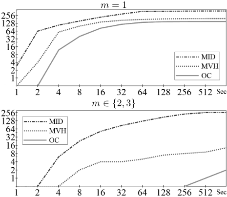
We generate instances for m = 2 and m = 3 by merging instances from the original benchmark. As a rule, we merge instances having the same size of time windows or the same gap between the time windows. Merged instances also have a similar number of airplanes. As m increases, we obtain instances with more airplanes. We implement our solution (denoted MID) using the Choco Solver and compare it against two implementations of the cumulative constraint that the solver provides. The first implementation performs an overload checking (denoted OC) in O(n log n) using a Θtree as designed by [Vil´ım, Bart´ak, & ˘Cepek, 2004]. The second implementation (denoted MVH) is an implementation of the edge-finder [Mercier & Hentenryck, 2008] in O(n2 ). Experiments are run arbitrarily on an Opteron 275 2.2 GHz and an Opteron 2376 2.3 GHz . Running times may vary depending on which processor executes the program.
Figure 1 shows that MID solves more problems in a given time for m ∈ {1, 2, 3} than MVH and OC. The difference in performance becomes more prominent as m increases. For m = 3, MID solves 134 instances in 20 minutes, MVH solves 3 instances, and OC solves none. Table 2 shows that MID solves the problem with significantly fewer backtracks. MVH performs fewer backtracks as n increases indicating that the filtering gets slower and fewer nodes are visited within 20 minutes.
8 Conclusion
We introduced the MULTI-INTER-DISTANCE constraint. We made the connection between this constraint and the properties of the shortest paths in the scheduling graph. We applied these properties in the design of the first filtering algorithm achieving bounds consistency. This new constraint is very successful at solving large instances of the runway scheduling problem. The theorems we proved about the MULTI-INTER-DISTANCE constraint may lead in the future to the design of better filtering algorithms for related constraints such as the INTER-DISTANCE and the CUMULATIVE constraints.
| m= 1 | m= 2 | m= 3 | ||||||||||||
|---|---|---|---|---|---|---|---|---|---|---|---|---|---|---|
| n | OC | MVH | MID | MVH | MID | MVH | MID | |||||||
| 15 | 94% | 999194 | 88% | 106325 | 17% | 22 | ||||||||
| 30 | 95% | 2755211 | 88% | 332083 | 16% | 333 | 100% | 722423 | 31% | 177 | ||||
| 45 | 97% | 2402617 | 97% | 306429 | 22% | 1040 | 100% | 322937 | 31% | 4607 | 100% | 376261 | 31% | 4 |
| 60 | 100% | 1583362 | 97% | 238024 | 22% | 1515 | 100% | 215728 | 15% | 543 | 100% | 213391 | 50% | 2840 |
| 75 | 98% | 1101707 | 94% | 152017 | 28% | 3111 | 100% | 129688 | 33% | 1436 | 100% | 120684 | 38% | 128 |
| 90 | 98% | 927161 | 98% | 106661 | 36% | 238 | 100% | 82496 | 29% | 4781 | 100% | 86733 | 33% | 61 |
| 105 | 100% | 66912 | 56% | 1619 | 100% | 60971 | 19% | 1532 | ||||||
| 120 | 100% | 58777 | 50% | 785 | 100% | 44511 | 25% | 2583 | ||||||
| 135 | 100% | 46525 | 25% | 1236 | 100% | 38623 | 44% | 451 | ||||||
| 150 | 100% | 29326 | 44% | 1324 | 100% | 27765 | 44% | 518 | ||||||
| 165 | 100% | 25181 | 47% | 775 | ||||||||||
8.1 Acknowledgments
We would like to thank Arnaud Malapert for his support with the Choco solver and the reviewers for helping us simplifying the proof of Theorem 3. This research is supported by a NSERC Discovery Grant.
@inproceedings{ijcai2011p112,
  title     = {The Multi-Inter-Distance Constraint},
  author    = {Ouellet, Pierre and Quimper, Claude-Guy},
  booktitle = {Proceedings of the Twenty-Second International Joint Conference on
               Artificial Intelligence, {IJCAI-11}},
  publisher = {AAAI Press/International Joint Conferences on Artificial Intelligence},
  editor    = {Toby Walsh},
  pages     = {629--633},
  year      = {2011},
  month     = {7},
  doi       = {10.5591/978-1-57735-516-8/IJCAI11-112},
  url       = {https://doi.org/10.5591/978-1-57735-516-8/IJCAI11-112},
}
TY - CPAPER TI - The Multi-Inter-Distance Constraint AU - Ouellet, Pierre AU - Quimper, Claude-Guy T2 - Proceedings of the Twenty-Second International Joint Conference on Artificial Intelligence, IJCAI-11 PB - AAAI Press/International Joint Conferences on Artificial Intelligence PY - 2011 SP - 629 EP - 633 DO - 10.5591/978-1-57735-516-8/IJCAI11-112 UR - https://doi.org/10.5591/978-1-57735-516-8/IJCAI11-112 ER -Copied
Machine-readable versions of this paper, for tools and AI agents:





