Large Hinge Width on Sparse Random Hypergraphs

1 Introduction

Constraint Satisfaction Problems (CSPs) cover many important NP-hard problems in AI research. In the past, there are two fruitful lines of research on CSPs. One is about structural decomposition; another is about randomCSPs. The start

∗Research supported by the National 973 Program of China (2010CB328103), the NSFC grants (60725207, 60821003 and 60973033), the Open Fund of the State Key Laboratory of Software Development Environment (SKLSDE-2010KF-0X), and the ARC Future Fellowship (FT0991787). We thank Yang Yuan for helpful contributions, and the unknown reviewers for helpful comments.

† Institute of Software, School of Electronics Engineering and Computer Science, Key Laboratory of High Confidence Software Technologies (Peking University), Ministry of Education, Peking University, Beijing 100871, China. Email: {lt,sukl}@pku.edu.cn.

‡State Key Laboratory of Software Development Environment, Beihang University, Beijing 100083, China.

§Corresponding author: Ke Xu (kexu@nlsde.buaa.edu.cn).

point of structural decomposition is to identify tractable subclasses of CSPs. The main results are in this form: CSPs with constraint hypergraphs of bounded structural width are tractable. In particular, all known structural decomposition based solvers run in time ||I||O(w) , where ||I|| is input size and w is a structural width such as the size of minimum loop-cutset, hingewidth, tree-width, querywidth, (fractional) hypertree width, spread-cut, etc. A plethora of structural decomposition methods have been developed and compared with each other [Gottlob et al., 2000; Cohen et al., 2008; Greco and Scarcello, 2010]. For a recent survey, see [Dechter, 2006]. On the other hand, the start point of random CSPs is to identify hard instances to serve as benchmarks, such as random instances around the satisfiability threshold of random CSPs [Cheeseman et al., 1991; Mitchell et al., 1992; Selman et al., 1996; Cook and Mitchell, 1997; Xu and Li, 2000; Gao and Culberson, 2007; Xu et al., 2007]. The main results are in this form: there is an easy-hard-easy transition around the satisfiability threshold of random CSPs, and the hardest instances are around the satisfiability thresholds. For a recent survey, see [Gomes andWalsh, 2006].

However, a rigorous link between phase transition and hardness of random instances is still unestablished. By rigorous link we mean that no polynomial time solver can exist at the satisfiability thresholds. This is still out of our current proof techniques. Instead, we might show some theoretical evidence for random instances around the satisfiability thresholds to be hard for some specific solvers. For example, in most structural decomposition methods, after finding a decomposition of the given CSP instance, the join operation is performed on constraint relations contained in each node of the decomposition, to formulate a new solution-equivalent tree-like CSP instance. Each decomposition of a CSP instance of large (i.e. unbounded) width contains a node with a large number of variables. Performing a join on all the variables in such a node is typically of high computational cost. Therefore, a large structural width around the satisfiability threshold can provide some theoretical evidence for these random instances to be hard for that kind of structural decomposition based algorithm.

The most popular structural width is tree-width, see e.g. [Kloks, 1994]. Gao is the first to study tree-width on random hypergraphs from considerations of Constraint Satisfaction and Bayesian Networks [Gao, 2003]. For other structural width related to CSPs, very little is known on random hypergraphs. In this paper, we show a large hinge width on sparse random hypergraphs. Hinge decomposition was introduced by [Gyssens and Paredaens, 1984; Gyssens et al., 1994] and was further investigated by e.g. [Gottlob et al., 2000; 2001; Cohen et al., 2008; Greco and Scarcello, 2010]. The standard hinge decomposition based algorithm also has a stage of hinge decomposition and a stage of join operation. Compared with tree-width, hinge width has two characters. First, hinge width and tree-width are incomparable, in the sense that there exists family of hypergraphs with bounded tree-width and unbounded hinge width, and vice versa [Gottlob et al., 2000]. Second, hinge width is efficiently computable [Gyssens et al., 1994], while tree-width is not.

We show that for random hypergraphs on n vertices, where each k-element subset of vertices is selected with probability p independently and randomly to be a hyperedge, when the total number of edges is O(n) or O(n lnn), the hinge width can grow linearly with or even asymptotically equal to the number of hyperedges. In particular, for every fixed positive integer k ≥ 2, when p = O ( 1 nk-1 ) and the expected number of edges m = O(n), the hinge width is Ω(m), when p = O ( lnn nk-1 ), the hinge width is m-O(m).

Some random CSPs have satisfiability thresholds on sparse random constraint hypergraphs. Two concrete examples are Model RB and Model RD [Xu and Li, 2000]. Benchmarks based on Model RB and Model RD have been successfully applied in CSP solver competitions since the year 2005, and in many research papers on algorithms. The large hinge width results provide further theoretical evidence on hardness of Model RB and Model RD, besides the known results in [Xu and Li, 2006; Xu et al., 2007].

We also conduct experiments on these and other kinds of random graphs with several hundreds vertices, including regular random graphs and power law random graphs. The experimental results show that hinge width can also grow linearly with the expected number of hyperedges on these different random graphs and match well with our asymptotic analysis on classical sparse random hypergraphs. These results may be of further interests such as in recent practice [Ans´otegui et al., 2007; 2008].

2 CSPs and RandomHypergraphs

A CSP instance is a triple (V, D, C), where

• V = {v1, . . . , vn} is a set of n variables;
• D is a finite set of values called domain, whose size |D| can be either fixed or increasing with n;
• C is a set of constraints, and each constraint Ci is a pair (Si, Ri), where
• Si is a k-tuple of variables, called constraint scope;
• Ri is a subset of Dk , called constraint relation.

A constraint Ci = (Si, Ri) is satisfied if the k-tuple of values assigned to variables in Si is contained in Ri. A solution to a CSP instance is an assignment of values to all the variables that satisfies all constraints. The constraint hypergraph of a CSP instance is a hypergraph with variables as vertices and constraint scopes as hyperedges. For more on CSPs, see e.g. [Dechter, 2003; Lecoutre, 2009].

The constraint hypergraphs of random CSPs are random hypergraphs. For any fixed k, we use G(n, p, k) to denote the probability space of k-uniform random hypergraphs, in which on n vertices, each k-element subset of vertices is selected with probability p independently at random as a hyperedge. When the total number of hyperedges is O(n) or O(n lnn), they are called sparse. G(n, p, 2) is exactly the Classical Erd¨os-R´enyi random graph model G(n, p) [Janson et al., 2000]. We say events Qn occur with high probability (w.h.p.), if limn→∞Pr (Qn) = 1, usually written as Pr (Qn) = o(1). We will need the following two lemmas.

Definition 1 Let G be a hypergraph with vertex set V (G) and edge set E(G), then a (χ, s)-separator of G is a partition (S,A,B) of V (G), such that

• |S| ≤ χs and |A|, |B| ≥ s;
• there is no edge connecting A and B.

Lemma 1 Let G ∈ G(n, p = c nk-1 , k). If ϵ > 0, ϵn is unbounded, χ > 0, s = tn, 0 < t ≤ 1 χ+2 , t may change with n, and c > k!(χt(1-ln(χt))+(ln 2)(1-χt)+ϵ) kt-(1+χ)k tk -k2 t2 > 0, thenwith high probability, no (χ, s)-separator of G exists.

Proof Under the given parameters, if there is a (χ, s)- separator with |S| < χs, then we can move some vertices from A or B to S, such that S = χs and the resulting partition is still a (χ, s)-separator. Thus we only need to show that with high probability, there is no (χ, s)-separator with |S| = χs. Denote by P the set of all such separators.

Consider a partition W = (S,A,B) with |S| = χs and |A| = a ≥ s. Every edge not connecting A and B is contained in A∪S or B∪S. By inclusion-exclusion principle, the number of such edges is (a+χs k ) + (n-a k ) - (χs k ). Let λ(a) = (nk) - (a+χs k ) - (n-a k ) + (χs k ) be the number of edges connecting A and B, then Pr(W ∈ P) = (1 - p)λ(a) . By union bound, Pr(P ̸= ∅) ≤ 2( n χs)∑(n-χs)/2 a=s (n-χs a )(1-p)λ(a) .

Proof Recall that nk = n(n - 1) · · · (n - k + 1). Approximating by the first two terms in expansion of nk , we have (nk) = nk k! ≥ nk-(∑k-1 j=0 j)nk-1 k! = nk-(k2)nk-1 k! . Similarly by the first three terms of (n - a)k , we have (n-a k ) = (n-a)k k! ≤ nk-(∑a+k-1 j=a j)nk-1+(k2)a2nk-2 k! ≤ nk-(ak+(k2))nk-1+k2 a2 nk-2 k! . Also (a+χs k ) = (a+χs)k k! ≤ (a+χs)k k! . So λ(a) ≥ aknk-1-k2 a2nk-2-(χs+a)k k! . For a ≥ s and for large n, the minimum is achieved at a = s. □

The following lemma gives a lower bound on |edges(U)| in terms of a lower bound on |U|. The use of Chernoff Bound (see i.e. [Mitzenmacher and Upfal, 2005; Janson et al., 2000]) is not necessary, but for sharp parameters.

Lemma 2 Let G ∈ G(n, p = c nk-1 , k) and the expected number of edges of G is m = (nk) c nk-1 = O(n). For any U ⊆ V (G), if |U| ≥ n- τn, 0 < τ < 1, δ > 0, ϵ > 0, ϵτn is unbounded and c > (1-lnτ+ϵ)kk τ k-1 ek ((1+δ) ln(1+δ)-δ) , then w.h.p., |edges(U )| ≥ m(1 - n13 ) - (1 + δ)( τ e k )k cn.

Proof Let S = {S ⊆ V (G)||S| = τn}. Let XS be the number of edges in subgraph induced by S.

Claim 3 |E(G)| ≥m(1-n13 ) with high probability.

By these claims and Definition 2, w.h.p., edges(U) ≥ |E(G)| - XS ≥ m(1 - n13 ) - (1 + δ)( τ e k )k cn. □

3 HingeWidth

Definition 3 [Gyssens et al., 1994; Gottlob et al., 2000] Let G be a hypergraph, H ⊆ E(G), and F ⊆ E(G) - H. ⋃ H is the set of all vertices in edges in H. Then F is called connected with respect to (w.r.t.) H if, for any two edges, e, f ∈ F, there is a sequence of edges e1, . . . , em, such that:

• e1 = e;
• ei ∩ ei+1 ̸⊆ ⋃ H, for i = 1, . . . ,m-1;
• em = f.

The maximal connected subsets of E(G) - H w.r.t. H is called connected component of E(G) - H w.r.t. H.

Definition 4 [Gyssens et al., 1994; Gottlob et al., 2000] Let G be a hypergraph, and let H be either E(G) or a subset of E(G) containing at least two edges. Let H1, . . . ,Hm be the connected components of E(G) -H w.r.t. H. Then H is called a hinge if, for i = 1, . . . ,m, there exists an edge hi ∈ H such that

Definition 5 [Gyssens et al., 1994; Gottlob et al., 2000] A hinge decomposition of hypergraph G is a tree T = (N, A), with nodes N and labeled arcs A, such that

1. the tree nodes are minimal hinges of G;
2. each edge inE(G) is contained in at least one tree node;
3. two adjacent tree nodes share precisely one edge which is the label of the arc connecting the two nodes; moreover, their shared variables are precisely the members of this edges;
4. the vertices of G shared by two tree nodes are entirely contained in each tree node on their connecting path.

It was shown in [Gyssens et al., 1994] that the cardinality of the largest node in any hinge decomposition of G is an invariant of G, which is the cardinality of the largest minimal hinge. We call it hinge width of G, and denote it by hw(G).

The following Algorithm 1 is from [Gyssens et al., 1994].

Input: A hypergraph G = (V, E)

Output: A hinge decomposition T for G

• 1: Mark each edge in E as unused. Set i = 0, N0 = {E} and A0 = ∅, and mark the node in N0 as non-minimal.
• 2: If all nodes of Ni are marked minimal, then set T = (Ni,Ai) and stop. Else choose a non-minimal node F in Ni .
• 3: If all edges in F are marked as used, then mark F as minimal and goto 2. Else, choose an unused edge e ∈ F and mark e as used.
• 4: Let Γ = {D ∪ {e}|D is a connected component of F - e with respect to e} and γ : F → Γ be any function such that for all f ∈ F, f ∈ γ(f). If |Γ| = 1, then goto 3.
• 5: Set

and mark all nodes newly added to Ni+1 as non-minimal. 6: Increment i and goto 2.

Algorithm 1: Computing a hinge decomposition

4 Asymptotic Analysis

A complete run from steps 2 to 6 in Algorithm 1 is called a round. For all round i, assume that Ni = {H (i) 1 , . . . ,H(i) pi }. Let H (i) max be the hinge in Ni with the maximum number of vertices | ⋃ H (i) max|. Suppose that Algorithm 1 stops when i = I. Then |H (I) max| is a lower bound of hw(G).

Definition 6 When step 5 is running, the edge e in steps 3 to 5 is called a separating edge [Gyssens et al., 1994]. Denote by ∂(H (i) j ) the set of all separating edges in H (i) j .

Proposition 1 For all i and j, there is no edge in G connecting V (G) - ⋃ H (i) j and ⋃ H (i) j - ⋃ ∂(H (i) j ).

Proof By steps 4 and 5 in Algorithm 1, except possibly by a separating edge, there is no other edge connecting vertices in ⋃ H (i) j1 and vertices in ⋃ H (i) j2 for j1 ̸= j2. □

To lower bound |H (I) max|, let U = ⋃ H (I) max - ⋃ ∂(H (I) max). By Definition 2 and Proposition 1, edges(U) ⊆ H (I) max. Thus hw(G) ≥ |H (I) max| ≥ |edges(U)|. Below we will first get an upper bound on I and a lower bound on |U| (Lemma 6), and then by Lemma 2 get a lower bound on |edges(U)|.

Lemma 3 For all i, | ⋃ H (i) max| ≤ n - i.

Proof For all i, we have the following three claims.

Claim 4 For all j, | ⋃ H (i) j | ≥ k +1.

Proof By Definition 4 about hinge, |H(i) j | ≥ 2. Two different k-uniformhyperedges have at least k +1 vertices. □

Proof Recall that (Ni,Ai) is a tree with pi hinge nodes and pi - 1 tree edges. By step 5 in Algorithm 1, every tree edge is labeled by a separating edge, and every pair of hinge nodes connected by a tree edge shares the separating edge. So in the sum ∑pi j=1 | ⋃ H (i) j |, separating edges are totally recounted by pi-1 times and each separating edge has k vertices. □

Claim 6 pi ≥ i +1.

Proof By induction. When i = 0, N0 = {E}, so p0 = 1. In each round, at step 5 in Algorithm 1, an old hinge is split into at least two new hinges, so pi+1 ≥ pi +1. □

Now by Claim 5, ∑pi j=1 | ⋃ H (i) j | ≤ n + (pi - 1)k. By Claim 4, ∑pi j=2 | ⋃ H (i) j | ≥ (pi - 1)(k + 1). By Claim 6, pi ≥ i + 1. Without lose of generality, we may assume that H (i) max = H (i) 1 , so | ⋃ H (i) max| = | ⋃ H (i) 1 | ≤ n+ (pi -1)k - (pi -1)(k +1) = n-pi +1 ≤ n- i. □

Lemma 4 For all i and s, if (k + 1)s ≤ | ⋃ H(i) max| ≤ n - s and i ≤ s, then there is a (k, s) - separator in G.

Proof Let S = ⋃ ∂(H (i) max), A = ⋃ H (i) max \ S, and B = V (G) \ ⋃ H (i) max. Clearly, (S,A,B) is a partition of V (G). Below we show that (S, A, B) is a (k, s)-separator of G.

Claim 7 For all i, |∂(H (i) max)| ≤ | ⋃pi j=1 ∂(H (i) j )| = i.

Proof At each round, exactly one new separating edge e is added to ⋃pi j=1 ∂(H (i) j ) at steps 3 to 5 in Algorithm 1. □

Now by Claim 7 and i ≤ s, |∂H (i) max| ≤ i ≤ s. Each hyperedge in ∂H (i) max has k vertices, so |S| ≤ ks. By | ⋃ H (i) max| ≥ (k + 1)s, |A| ≥ (k + 1)s - ks = s. By | ⋃ H (i) max| ≤ n - s, |B| ≥ n - (n - s) = s. By Proposition 1, no edge connects A and B. □

Lemma 5 For all i and s, if | ⋃ H(i) max| < (k + 1)s < n and i ≤ s < n 2k+3 , then there is a (k, s) - separator in G.

Proof Since | ⋃pi j=1 (⋃ H (i) j )| = |V (G)| = n, there is a j0 such that (k + 1)s ≤ | ⋃j0 j=1 (⋃ H (i) j )|. Since s < n 2k+3 , n-s > 2(k+1)s. By | ⋃ H (i) max| < (k+1)s, we can assume that | ⋃j0 j=1 (⋃ H (i) j )| ≤ n - s. Let S = ⋃j0 j=1 (⋃ ∂(H (i) j )), A = ⋃j0 j=1 (⋃ H (i) j ) \ S, and B = V (G) \ ⋃j0 j=1 (⋃ H (i) j ). The remaining part is similar to the proof of Lemma 4. □

Lemma 6 Let G ∈ G(n, p = c nk-1 , k). For any s = tn and 0 < t < 1 2k+3 , if c satisfies the conditions in Lemma 1, then I < s and |U| > n - (k + 1)s with high probability.

Proof By following three claims.

Claim 8 For all i ≤ s, | ⋃ H (i) max| > n - s with high probability.

Proof Otherwise by Lemma 4 and Lemma 5, with nonvanishing probability there is a (k, s)-separator of G, contradiction to Lemma 1. □

Claim 9 I < s with high probability.

Proof By Claim 8, | ⋃ H (s) max| > n - s. If I ≥ s, then by Lemma 3, | ⋃ H (s) max| ≤ n- s, a contradiction. □

Claim 10 |U| > n- (k + 1)s with high probability.

Proof By Claim 9 and Claim 8, | ⋃ H(I) max| > n - s. By Claim 7 and Claim 9, |∂(H (I) max)| ≤ I < s. Each edge in G has k vertices, so | ⋃ ∂(H (I) max)| < ks. Thus, |U| = | ⋃ H(I) max| - | ⋃ ∂(H (I) max)| > n- (k +1)s. □

This finishes the proof of Lemma 6. □

Theorem 1 Let G ∈ G(n, p = c nk-1 , k) and the expected number of edges of G is m = (nk) c nk-1 = O(n). If s = tn, 0 < t ≤ 1 2k+3 , ϵ > 0, ϵtn is unbounded, δ > 0, c > k!(kt(1-ln(kt))+(ln2)(1-kt)+ϵ) kt-(1+k)k tk-k2 t2 > 0 and c > (1-ln((k+1)t)+ϵ)kk [(k+1)t]k-1 ek [(1+δ) ln(1+δ)-δ] , then w.h.p., hw(G) = Ω(m).

Proof Set τ = (k + 1)t, we can easily check that the parameters satisfy conditions in Lemma 6 and Lemma 2. Thus by discussions at the beginning of this section, with high probability hw(G) ≥ |H (I) max| ≥ |edges(U)| = Ω(m). □

Theorem 2 Let G ∈ G(n, p = b ln n nk-1 , k) and the expected number of edges of G is m = (nk) b ln n nk-1 = O(n lnn). For any b > 0, hw(G) = m - o(m) with high probability.

Proof Similar to proof of Theorem 1. First, let s = tn, t = ( (ln2)(k-1)! b + ϵ) 1 lnn for any constant ϵ > 0, then all conditions in Lemma 6 are satisfied. Next, let c = b lnn, τ = (k + 1)t = d ln n where d = (k + 1) ( (ln 2)(k-1)! b + ϵ), and δ = (lnn)k-1 , then all conditions in Lemma 2 are satisfied. Finally, |edges(U)| ≥m(1-n13 )-(1+δ)( τe k )k cn = m(1 - n13 ) - 1+(ln n)k-1 (lnn)k ( de k )k cn =m- o(m). □

5 Model RB andModel RD

Two concrete random CSPs to apply Theorem 2 are Model RB and Model RD [Xu and Li, 2000]. Model RB is like this:

• given n variables each with domain {1, 2, ..., d}, where d = nα and α > 0 is constant;
• select with repetition m = rn lnn random constraint scopes, for each scope select without repetition k of n variables, where k ≥ 2 is an integer constant;
• select uniformly at randomwithout repetition (1-p)dk compatible assignments for each constraint, where 0 < p < 1 is constant.

In Model RD, in the last step above, each assignment for the k variables is selected with probability 1 - p as compatible independently. Model RB and Model RD have satisfiability thresholds rcr = - α ln(1-p) [Xu and Li, 2000]. A large hinge width result will provide further theoretical evidence on hardness of Model RB and Model RD, besides the known results in [Xu and Li, 2006; Xu et al., 2007].

Clearly Model RB and Model RD have the same space of random constraint hypergraphs, with constraint scopes as hyperedges. Let GRB (n, r, k) denote the probability space of these random constraint hypergraphs. We show an asymptotic equivalence between GRB (n, r, k) and G(n, p, k) for p = rn lnn/(nk) = O(lnn)/nk-1 , so that Theorem 2 can be applied to Model RB and Mode RD. We use the Ball and Bin model [Mitzenmacher and Upfal, 2005]. Suppose that we put a balls independently and uniformly at random into b bins. Then the joint distribution of the number of balls in each bin is referred to as in the exact case. In another case called the Poisson case, the number of balls in each bin is independent and has Poisson distribution with mean a/b.

Lemma 7 [Mitzenmacher and Upfal, 2005] Any event occurring with probability p in Poisson case occurs with probability at most pe√a in exact case.

Lemma 8 Let Qn be an arbitrary graph property, r > 0 and p = rn lnn/(nk). Then PrGRB (n,r,k) (Qn) ≤ e√rn ln n PrG(n,p,k) (Qn).

Proof Treating edges as balls and all k-element subsets of vertices as bins, then GRB (n, r, k) is no more than the exact case where a = rn lnn and b = (nk), and Poisson case is equivalent to G(n, p, k) with p = rn lnn/(nk). Then this lemma follows from Lemma 7. □

Corollary 1 Let G ∈ GRB (n, r, k). Then for any constant r > 0, with high probability, hw(G) = rn ln n - O(n).

Proof By Theorem 2 and the fact that all o(1)'s in its proofs are something like e-ϵn, which can subsume the e√rn lnn factor in the Lemma 8. □

6 Experiments

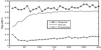
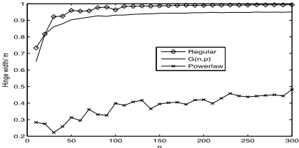
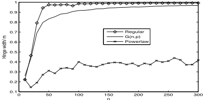
We do experiments on instances of a realistic size for different kinds of random graphs to complement the asymptotic analysis. For simplicity, we only consider graphs, i.e. k = 2. We let the number of vertices n increase from 10 to 300 with step length 10, and let the (expected) number of edges m be n, 2n and 0.4n lnn, respectively. At each pair (n,m), we generate 60 instances to average on hw/m, where hw is hinge width. We compare the results on classical random graphs G(n, p), regular random graphs and power law random graphs. We use the configuration model [Janson et al., 2000] to generate regular or power law instances with a given sequence of degrees. The results are displayed in Figures 1 to 3.

n

n

Figure 3: Results for m = 0.4n ln n

From the figures, we can find that on all these random graphs, hinge width hw grows linearly with the number of edges m. For each pair (n,m), regular random graphs have the largest hinge width, while power law random graphs have the smallest hinge width. Hinge width is also called the degree of cyclicity of graphs [Gyssens et al., 1994], graphs with more nodes of degree 1 or 2 will have smaller hinge width. Power law graphs do have more nodes of smaller degrees than regular graphs or G(n, p). Moreover, the experimental results match well with asymptotic analysis on G(n, p) already on instances of 100 to 300 vertices.

7 Conclusion and Future Work

We have shown that hinge width can grow linearly on sparse classical random hypergraphs. This provides theoretical evidence for random instances around the satisfiability thresholds to be hard for the standard hinge decomposition method, at least for Model RB and Model RD. We also conduct experiments on instances of a realistic size and the results match well with the asymptotic analysis. The hinge width in regular random graphs is the largest among all three kinds of random graphs, so this result supports the previous suggestions to use balanced random instances as benchmarks [Ans´otegui et al., 2007; 2008]. More interestingly, the hinge width in power law graphs is much lower than that in regular/classical random graphs. Since the power law graphs are more common in the real world, this implies that the hinge decomposition is still of potential use in the real-world instances. Our analysis and experiments depend essentially on the efficient hinge algorithm (Algorithm 1) given by [Gyssens et al., 1994]. Thus tools developed in structural decomposition are useful, not only in solving restricted easy CSP instances, but also in analyzing random hard CSP instances. For other structural width, such as (fractional) hypertree width and spread-cut, a similar analysis or experiment on random instances should be an interesting future work. But this seems to be a challenge task. For example, we can easily handle hinge width on 1, 000 vertices, but can hardly handle tree-width exactly on more than 50 vertices, due to a lack of efficient tree-width algorithms.