
An Efficient Nonnegative Matrix Factorization Approach in Flexible Kernel Space
Proceedings of the Twenty-First International Joint Conference on Artificial Intelligence. Pages 1345-1349.
© 2009 International Joint Conferences on Artificial Intelligence
Abstract
In this paper, we propose a general formulation for kernel nonnegative matrix factorization with flexible kernels. Specifically, we propose the Gaussian nonnegative matrix factorization (GNMF) algorithm by using the Gaussian kernel in the framework. Different from a recently developed polynomial NMF (PNMF), GNMF finds basis vectors in the kernel-induced feature space and the computational cost is independent of input dimensions. Furthermore, we prove the convergence and nonnegativity of decomposition of our method. Extensive experiments compared with PNMF and other NMF algorithms on several face databases, validate the effectiveness of the proposed method.Daoqiang Zhang, Wanquan Liu
- [Berry et al., 2007] M. Berry, M. Browne, A. Langville, V. Pauca, and R. Plemmons. Algorithms and applications for approximate nonnegative matrix factorization. Compu- tational Statistics & Data Analysis, 52:155-173, 2007.
- [Buciu et al., 2008] I. Buciu, N. Nikolaidis, and I. Pitas. Nonnegative matrix factorization in polynomial feature space. IEEE Trans. on NN, 19(6):1090-695, 2008.
- [Hoyer, 2004] P.O. Hoyer. Non-negative matrix factorization with sparseness constraints. Journal of Machine Learning Research, 5:1457-1469, 2004.
- [Lee and Seung, 1999] D.D. Lee and H.S. Seung. Learning the parts of objects by nonnegative matrix factorization. Nature, 401:788-791, 1999.
- [Lee and Seung, 2001] D.D. Lee and H.S. Seung. Algo- rithms for non-negative matrix factorization. In NIPS, vol- ume 13, pages 629-634, 2001.
- [Li et al., 2001] S. Li, X. Hou, H. Zhang, and Q. Cheng. Learning spatially localized, parts-based representation. In CVPR, pages 207-212, 2001.
- [Lin, 2007] C.J. Lin. Projected gradient methods for non- negative matrix factorization. Neural Computation, 19(10):2756-2779, 2007.
- [Pascual-Montano et al., 2006] A. Pascual-Montano, J.M. Carazo, K. Kochi, D. Lehmann, and R.D. Pascual-Marqui. Non-smooth non-negative matrix factorization (nsnmf). IEEE Trans. on PAMI, 28(3):403-415, 2006.
- [Shawe-Taylor and Cristianini, 2004] J. Shawe-Taylor and N. Cristianini. Kernel Methods for Pattern Analysis. Cam- bridge University Press, 2004.
- [Yang et al., 2008] J. Yang, S. Yan, Y. Fu, X. Li, and T. Huang. Non-negative graph embedding. In CVPR, pages 1-8, 2008.
- [Zafeiriou et al., 2006] S. Zafeiriou, A. Tefas, I. Buciu, and I. Pitas. Exploiting discriminant information in nonneg- ative matrix factorization with application to frontal face verification. IEEE Trans. on NN, 17(3):683-695, 2006.
- [Zhang et al., 2006] D. Zhang, Z.H. Zhou, and S. Chen. Non-negative matrix factorization on kernels. In PRICAI, pages 404-412, 2006.
References were extracted automatically from the PDF and may contain errors.
Full text extracted automatically from the PDF; figures, tables and equations may differ. The PDF is the version of record.
1 Introduction
Nonnegative matrix factorization (NMF) is a recent linear method for finding low-dimensional representation of nonnegative high-dimensional data such as images and texts. It imposes the nonnegativity constraints in both its basis vectors (bases) and coefficients. Due to its part-based representation property [Lee and Seung, 1999], NMF and its variations have been applied to a variety of applications, such as image classification, face expression recognition, face and object recognition, document clustering, etc [Berry et al., 2007].
Over the last decade, many variants on NMF have been proposed to improve original NMF from different perspectives. To our knowledge, most works focus on one or several of the following aspects: 1) enhancing the sparseness of representation [Li et al., 2001][Hoyer, 2004][Pascual-Montano et al., 2006]; 2) investigating alternative computational solutions [Berry et al., 2007][Lin, 2007]; 3) introducing discriminative information to improve classification power [Zafeiriou et al., 2006][Yang et al., 2008]. For example, to enhance the sparseness, Li et al. [2001] and Hoyer [2004] imposed different extra constraints. As for alternative computational solutions, besides the well-known multiplicative update algorithms, Lin [2007] recently proposed the projected gradient methods for NMF based on bound-constrained optimization.
∗This work is partially supported by NSFC (60875030), Doctoral Fund of MOE (200802870003) and Australia ARC Linkage grant.
At last, Zafeiriou et al. [2006] and Yang et al. [2008] both introduced discriminant information into NMF for better classification power.
On the other hand, NMF and its many variants are linear models, i.e. data are decomposed as a linear mixture of basis vectors. Recently, kernel methods [Shawe-Taylor and Cristianini, 2004] have been used in NMF to deal with nonlinear correlation in data. Buciu et al. [2008] proposed the polynomial nonnegative matrix factorization (PNMF) method, where the original data as well as the unknown basis vectors are first transformed by a nonlinear polynomial kernel mapping into a higher feature space and then a nonnegative decomposition is accomplished in the feature space. Although PNMF shows improved classification power over conventional NMF algorithms, there remain several problems unresolved yet. Firstly, only the polynomial kernel function can be used in PNMF to keep the nonnegativity constraint. Other kernel functions such as the well-known Gaussian kernel may not be adopted because of the negative solution resulting from the derivative associated from the Gaussian kernel. Secondly, although the decomposition is performed in feature space, PNMF still seeks basis vectors in the original input space and then transform them into feature space. It remains unknown how to find basis vectors directly in the feature space. Finally, at each iteration step of PNMF, the kernel matrices have to be recomputed, and thus a great deal of computational cost are required. In our previous work, we ever proposed performing NMF directly on kernel matrices, but rigorous derivation and analysis in theory was not given [Zhang et al., 2006].
In this paper, we propose an alternative way for using kernel method in NMF. A general framework for kernel based NMF is presented which can efficiently use flexible kernel functions. Besides, unlike in PNMF where basis vectors are still found in original input space, our method directly seeks bases in transformed feature space, which can be further changed into a much easier kernel decomposition problem by using kernel functions. Furthermore, there is no need to repeatedly compute the kernel matrices in each iteration, and the computational cost is low. Algorithmic convergence and nonnegativity property are guaranteed by theoretical proof. Specifically, we use the Gaussian kernel in our framework and present the Gaussian nonnegative matrix factorization (GNMF) algorithm. The effectiveness of the proposed method is validated by extensive experiments on several face databases compared with PNMF and conventional NMF algorithms.
The rest of this paper is organized as follows. Section 2 reviews the standard NMF algorithm and the recently proposed PNMF algorithm. Then in Section 3, we present the flexible kernel based NMF framework and give the proposed GNMF algorithm in detail. Experimental results on several benchmark face databases are reported in Section 4. And finally, we conclude this paper and indicate some issues for future research in Section 5.
Notations: Throughout this paper, we use lowercase bold letters to denote vectors and uppercase bold letters to denote matrices, if not stated specially. The operator 〈·〉 means the inner product, and ‖ · ‖ denotes the Frobenius norm. AT denotes the transpose of a matrix A, A+ indicates the MoorePenrose pseudo-inverse of matrix A, and tr(A) means the trace operator of the corresponding matrix A. The symbol Ai· denotes the ith row vector of matrix A, and A·i means the ith column vector of matrix A. X ≥ 0 represents the matrix is nonnegative.
2 NMF and PNMF
2.1 NMF
The key ingredient of NMF is the non-negativity constraints imposed on the two matrix factors. Assume that the observed data of the objects are represented as an n×mmatrix X, each column of which contains n non-negative attribute values in one of the m objects. In order to represent data or reduce the dimensionality, NMF finds two non-negative matrix factors W and H such that X ≈ WH. In general, the standard NMF problem can be formally expressed as follows [Lee and Seung, 2001]:
Problem 1 (The NMF problem) Given an n × m nonnegative matrix X and a positive integer r < min{n,m}, find nonnegative matrices W and H to minimize the following objective function
In order to obtain W and H, a multiplicative update rule is given in [Lee and Seung, 2001].
2.2 PNMF
The standard NMF is a linear model, and thus it only allows linear correlation. To handle the nonlinear correlation, the polynomial NMF (PNMF) algorithm was recently proposed. The main idea of PNMF is to first transform data into higher dimensional feature space by using a polynomial kernel-induced nonlinear mapping and then perform decomposition in that feature space. Let φ denote the nonlinear mapping corresponding to the polynomial kernel, i.e. k(x, z) = 〈x, z〉{d} = 〈φ(x), φ(z)〉, then the PNMF problem can be formally expressed as follows [Buciu et al., 2008]:
Problem 2 (The PNMF problem) Given the nonnegative input data X = [x1, x2, ..., xm] and the corresponding transformed input data in polynomial feature space Φ(X) =
[φ(x1), φ(x2), ..., φ(xm)], and a positive integer r, find nonnegative matrices W = [w1, w2, ..., wr ] and H to minimize the following objective function
where Y
= [φ(w1), φ(w2), ..., φ(wr)].
It is easy to see that if we expand the objective function in Eq. 2, the PNMF problem can be solved by invoking only the kernel function. In order to obtainW andH, a multiplicative update rule is given as follows [Buciu et al., 2008]:
where (Kwx)aμ = k(wa, xμ), (Kww)ab = k(wa,wb) are kernel matrices of dimensions r × m and r × r, respectively. (K′xw)ia = k′ (xi,wa), (K′ww)ab = k′ (wa, wb) are kernel matrices of dimensions m × r and r × r respectively, wherek′ is the derivative of the polynomial kernel k, i.e. k′ (x, z) = d〈x, z〉{d-1} . Λ is a diagonal matrix whose diagonal elements are λaa = ∑mj=1 Haj .
It is noteworthy that although PNMF has used the kernel method to handle nonlinear correlations, it is restricted with the polynomialhkn kernel functions. That is because the iteration updating rule (Eq. 4) needs to compute the derivative of a kernel, while most kernel functions such as the Gaussian kernel may have negative derivatives and thus cannot remain the nonnegativity property in the decomposition. This motivates us to find alternative ways to allow more flexible kernel functions in NMF.
3 The ProposedMethod
To overcome the limitations of PNMF, in this section, we propose an alternative kernel NMF framework with flexible kernels. In the following, we first give the new problem formulation, and then derive the iterative update rules and prove the convergence. Specifically, we use the Gaussian kernel in the framework and give the Gaussian NMF (GNMF) algorithm in detail at the end of this section.
3.1 Problem Formulation
Assume that the observed data of the objects are represented as an n × m matrix X = [x1, x2, ..., xm]. Let φ be an implicit nonlinear mapping from the original input space to a high-dimensional feature space, where the inner product is defined as a kernel k(x, y) = 〈φ(x), φ(y)〉 in the original input space. Denote Φ(X) = [φ(x1), φ(x2), ..., φ(xm)]. Like in NMF, we want to find two non-negative matrix factors W and H such that Φ(X) ≈ WH. However, because the explicit form of φ is unknown and φ(xi) may lie in very high or even infinite dimensional space, it is unpractical to directly decompose Φ(X) in the feature space.
Fortunately, we can solve that problem by representing the basis vectors wi with linear combinations of transformed data φ(x1), φ(x2), ..., φ(xm), i.e. wi = ∑mj=1 Ajiφ(xj) = Φ(X)A·i, i = 1, ..., r. Denote W = Φ(X)A, we have
where K = ΦT (X)Φ(X) is the kernel matrix. Note that each column vector of W lies in the kernel-induced feature space, and thus we cannot constrain it explicitly. Instead, we approximately constrain AT KA ≥ 0 due to W T W = AT ΦT (X)Φ(X)A = AT KA ≥ 0. From Eq. 5, the flexible-kernel NMF problem can be expressed as follows:
Problem 3 (The Flexible-Kernel NMF problem) Given the nonnegative input data X = [x1, x2, ..., xm] and the corresponding kernel matrix K = ΦT (X)Φ(X), and a positive integer r, find A and nonnegative matrix H to minimize the following objective function
It is easy to see that in the flexible-kernel NMF problem, basis vectors are sought in the transformed feature space, which is apparently different from the PNMF problem. On the other hand, the objective function in Eq. 6 is biquadratic, and generally there is no closed-form solution for it. In the next subsection, we will present an alternately iterative procedure for computing the nonnegative solution.
3.2 Iterative Update Procedure
Before formally describing the derivations of the iterative update rule, we first introduce some preliminary concepts and lemmas which will be used later.
Definition 1 (Auxiliary function) Function G(A,A′ ) is an auxiliary function for function F (A) if the conditions
G(A, A′
) ≥ F
(A), G(A, A) =
F
are satisfied.
Lemma 1 [Lee and Seung, 2001] If G is an auxiliary function, then F is nonincreasing under the update
where t denotes the t-th iteration.
Solution of H for given A
When A is fixed, the objective function in Eq. 6 with respect to the coefficient matrix H = [H·1,H·2, ...,H·m] can be rewritten as
(A)
(7)
From Eq. 9, it is easy to notice that different column vectors of H are independent to each other for optimization, and thus the objective function can be further simplified into column-wise form as
Following [Lee and Seung, 2001], we can construct an auxiliary function of F (H·i) in Eq. 10 as below.
Lemma 2 If L(Ht ·i ) is the diagonal matrix
where δab is the indicator function, then
is an auxiliary function of F (H·i) in Eq. 10.
The proof for Lemma 2 is similar as that in [Lee and Seung, 2001] and we omit it due to space limit. Then, according to Lemma 1, Ht+1 ·i can be computed by minimizing G(H·i, Ht ·i ).
From Eqs. 10 and 11, and after some algebra operations, we obtain the update rule for Hai as
Solution of A for given H
When H is fixed, we want to optimize A according to the objective function in Eq. 6. For that purpose, we introduce an auxiliary matrix B = K 12A, where K is the kernel matrix. However, there may be a few negative components in matrix K 12 . To keep the nonnegativity property, in this paper we project those negative values to the nearest nonnegative value, i.e. 0, and obtain both symmetric and nonnegative matrix K 12 . In our experiments, we found that only very few components of K 12 are of negative values and the projection method works very well in practice.
From B = K 12A, we have A = (K 1 2 )-1B, then the objective function in Eq. 6 with with respect to the matrix B = [BT 1· , BT 2· , ...,BTm·]T can be rewritten as
From Eq. 15, it is obvious that different row vectors of B are independent to each other for optimization, and thus the objective function can be further simplified into row-wise form as
Similarly, we can construct an auxiliary function of F (Bi· ) in Eq. 16 as below.
Lemma 3 If L(Bt i· ) is the diagonal matrix
where δab is the indicator function, then
is an auxiliary function of F (Bi·) in Eq. 16.
Also, it is easy to prove Lemma 3 following [Lee and Seung, 2001]. Similarly, according to Lemma 1, Bt+1 i· can be computed by minimizing G(Bi· , Bt i· ).
From Eq. 16 and Eq. 17, and after some algebra operations, we obtain the update rule for Bia as
It is obvious that Bt+1 is nonnegative if the matrices H and Bt are nonnegative. After B is obtained, we update the matrix A as
Equations 20, 21 and 14 constitute the iterative update procedure, which optimizes the matrices H and A alternatively. In the next subsection, we will prove the iterative update procedure can converge to a local optimum.
3.3 Convergence Proof
In this section, we prove the convergence of the iterative update procedure proposed in last subsection.
The iterative update procedure between H and A can be further transformed the iterative update between H and B. Substituting Eq. 21 into Eq. 14, we have
Now the iterative update procedure consist of Eqs. 22 and 20. From Eq. 22, the updated matrix Ht+1 is still nonnegative if the matrices B and Ht are nonnegative.
Theorem 1 The alternative iterative update procedure
converges to a local optimum.
Proof. Following [Lee and Seung, 2001] and [Yang et al., 2008], we define
From the update rule for B, we have
Similarly, from the update rule for H, we have
On the other hand, from Eq. 5, it is easy to notice that F (Bt , Ht ) ≥ 0. Then, F (Bt , Ht ) decreases monotonically and has lower bound, and hence F (Bt ,Ht) will converge to a local optimum. □
3.4 The GNMF Algorithm
In this section, we summarize the above analysis by presenting a specific Gaussian NMF (GNMF) algorithm by using the Gaussian kernel in the flexible-kernel NMF framework. However, it is noteworthy that our method is not confined to the Gaussian kernel, and any kind of kernels can be used. Algorithm 1 lists the GNMF algorithm in detail.
Algorithm 1: The GNMF algorithm
Input:
Kernel matrix {Kij = exp(-
A positive integer r < m
A small threshold ε > 0.
Initialize:
Perform SVD decomposition K = USU T
Generate initial nonnegative matrices B0 and H0 with dimensions m × r and r × m respectively.
For t = 1, ..., tmax
1. For givenH = Ht , update the matrix B as
2. For givenB = Bt , update the matrix H as
Output:
4 Experiments
In this section, we test the performance of the proposed flexible-kernel NMF method. We first compare the GNMF algorithm with standard NMF, Localized NMF (LNMF) and PNMF. Also, we replace the Gaussian kernel in our GNMF with polynomial kernel (pKNMF) and compare its performance. All the NMF algorithms use the same stopping condition (see Step 3 in Algorithm 1) and ε is set to 10-4, and the maximum iteration steps tmax is set to 500 in all experiments. For completeness, we also report results of kernel principal component analysis with both the Gaussian kernel (gKPCA) and polynomial kernel (pKPCA).
‖xi-xj ‖2
2σ2 )}mi,j=1
4.1 Data Sets and Experimental Config
In our experiments, we use 4 benchmark face databases, i.e. AR, FERET, ORL and Yale. The AR database contains 1400 frontal facial images from 100 persons, each of which has 14 images at 2 different stages. The FERET database used in our experiments contains 200 persons, each with 2 images. The ORL database consists of 40 persons, each with 10 images. The Yale database contains 165 images from 11 persons. For each database, we resize images in 3 different scales, i.e. 66x48, 33x24 and 16x12 for AR, 60x60, 32x32 and 16x16 for FERET, 64x64, 32x32 and 16x16 for both ORL and Yale. So, there are totally 12 databases for experiments.
We evaluate performances of different algorithms using recognition accuracy. For each database, the first half of the images from each person are used for training and and the rest for testing. The Nearest Neighborhood classifier is adopted for classification after dimensionality reduction, where the number of reduced dimensions is set as mn/(m + n), if without extra explanations. For PNMF, pKNMF and GNMF as well as pKPCA and gKPCA, crossvalidation is used for selecting the kernel parameters d and σ respectively. For pKNMF and GNMF, features of a test image xte are extracted as (Φ(X)A)+φ(xte) ≈ A+(Φ(X))+ (ΦT (X))+ΦT (X)φ(xte) = A+K-1Kte, where Kte = ΦT (X)φ(xte). All experiments are carried out on a PC with 2.7GHz CPU and 1GB RAM.
4.2 Experimental Results
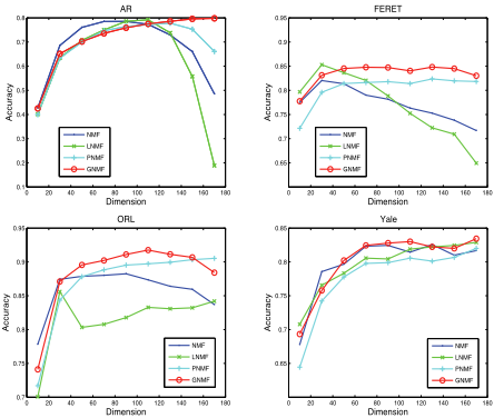
We first compare GNMF with NMF, LNMF, PNMF, and Table 1 gives the classification accuracies of under fixed dimensions (r = mn/(m + n)) on the 12 databases. It can be seen from Table 1 that GNMF outperforms the other three algorithms in most cases and is consistently superior to PNMF. Table 1 also indicates that in most cases (except on AR) the four algorithms achieve better performances on small image size than large ones. Furthermore, Fig. 1 gives the classification accuracies of the four algorithms when different number of dimensions are used. We can see from Fig. 1 that GNMF outperforms other algorithms in most cases and is more robust to variations on dimensions.
| Data sets | NMF | LNMF | PNMF | GNMF |
|---|---|---|---|---|
| AR-16x12 | 67.16 | 60.29 | 75.46 | 79.26 |
| AR-33x24 | 79.51 | 85.69 | 82.51 | 84.67 |
| AR-66x48 | 77.69 | 87.73 | 80.31 | 81.17 |
| FERET-16x16 | 76.7 | 75.2 | 82.6 | 84.95 |
| FERET-32x32 | 72.55 | 73.6 | 80.4 | 83.25 |
| FERET-60x60 | 65.65 | 73.5 | 79.65 | 82.5 |
| ORL-16x16 | 88.25 | 82.75 | 90.65 | 91.7 |
| ORL-32x32 | 86.2 | 81.45 | 87.75 | 89.15 |
| ORL-64x64 | 81.7 | 80.3 | 83.75 | 85.25 |
| Yale-16x16 | 82.44 | 82.44 | 81.22 | 83.11 |
| Yale-32x32 | 80.78 | 81.78 | 81.78 | 83.0 |
| Yale-64x64 | 77.89 | 81.89 | 80.67 | 82.56 |
| Average | 78.04 | 78.89 | 82.23 | 84.21 |
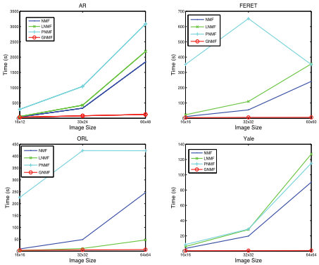
We also investigate the computational costs of four algorithms. It is easy to derive that the computational complexity for the iterative procedure of GNMF is O(m2 rt), where m is the data size, r is the reduced dimensions and t is the iteration numbers. In comparison, the complexities of NMF and PNMF are O(nmrt) and O(nmrdt), where n is data dimensions and d is the order of polynomial kernel. Figure 2 plots the curves of running time vs. different image sizes for the four algorithms. As we expected, the curves of GNMF is nearly horizontal on all databases because its computational complexity is not dependent on the image size, i.e. n. Figure 2 shows that GNMF is much efficient than the other algorithms, especially for high-dimensional cases.
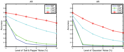
On the other hand, due to the use of kernel functions both PNMF and GNMF can deal with nonlinear correlations between basis vectors and thus are potentially more robust to image noises than their linear competitors. We carry out experiments on AR database when the test images are corrupted by different levels of 'Salt & Pepper' and 'Gaussian' noises respectively. Figure 3 gives the classification accuracies of four algorithms when test images are corrupted by different levels of noises. Figure 3 validate that nonlinear methods PNMF and GNMF are more advantageous for enhancing robustness to image noises than both NMF and LNMF, and GNMF consistently outperforms PNMF in both cases.
Finally, we make comparisons between kernel NMF (including pKNMF and GNMF) and kernel PCA (including pKPCA and gKPCA), and the results are given in Table 2. Table 2 indicates that pKNMF and GNMF achieve better averaged accuracies than pKPCA and gKPCA respectively across 12 databases, which validates the usefulness of kernel NMF. Furthermore, contrasting Table 2 with Table 1, it can be seen that our pKNMF outperforms PNMF in most cases and achieves better averaged accuracy.
5 Conclusion
In this paper, we proposed a general flexible-kernel based framework for nonnegative matrix factorization. We derived an alternative iteration update procedure and proved its convergence. Specifically, we proposed the Gaussian NMF (GNMF) algorithm with the Gaussian kernel and evaluated its performances on several face databases. One extra advantage of our method is that its computational complexity is independent on data dimensions and thus is potential for high-dimensional data decomposition. Moreover, GNMF can be used for negative data decomposition due to the Gaussian kernel transform and we will investigate that issue in future. Another future work is exploiting supervision information in GNMF to further enhance the discriminant power.
Acknowledgments We thank the the anonymous reviewers for their helpful comments and suggestions.
@inproceedings{ijcai2009p226,
  title     = {An Efficient Nonnegative Matrix Factorization Approach in Flexible Kernel Space},
  author    = {Zhang, Daoqiang and Liu, Wanquan},
  booktitle = {Proceedings of the Twenty-First International Joint Conference on
               Artificial Intelligence, {IJCAI-09}},
  publisher = {International Joint Conferences on Artificial Intelligence},
  editor    = {Craig Boutilier},
  pages     = {1345--1349},
  year      = {2009},
  url       = {https://ijcai.org/proceedings/2009/226},
}
TY - CPAPER TI - An Efficient Nonnegative Matrix Factorization Approach in Flexible Kernel Space AU - Zhang, Daoqiang AU - Liu, Wanquan T2 - Proceedings of the Twenty-First International Joint Conference on Artificial Intelligence, IJCAI-09 PB - International Joint Conferences on Artificial Intelligence PY - 2009 SP - 1345 EP - 1349 UR - https://ijcai.org/proceedings/2009/226 ER -Copied
Machine-readable versions of this paper, for tools and AI agents:





