
Multi-Relational Learning with Gaussian Processes
Proceedings of the Twenty-First International Joint Conference on Artificial Intelligence. Pages 1309-1313.
© 2009 International Joint Conferences on Artificial Intelligence
Abstract
Due to their flexible nonparametric nature, Gaussian process models are very effective at solving hard machine learning problems. While existing Gaussian process models focus on modeling one single relation, we present a generalized GP model, named multi-relational Gaussian process model, that is able to deal with an arbitrary number of relations in a domain of interest. The proposed model is analyzed in the context of bipartite, directed, and undirected univariate relations. Experimental results on real-world datasets show that exploiting the correlations among different entity types and relations can indeed improve prediction performance.Zhao Xu, Kristian Kersting, Volker Tresp
- [Carbonetto et al., 2005] P. Carbonetto, J. Kisynski, N. de Freitas, and D. Poole. Nonparametric bayesian logic. In Proc. 21st Conf. on Uncertainty in AI (UAI), 2005.
- [Chu et al., 2006] W. Chu, V. Sindhwani, Z. Ghahramani, and S. Keerthi. Relational learning with gaussian pro- cesses. In Neural Information Processing Systems, 2006.
- [De Raedt, 2008] L. De Raedt. Logical and Relational Learning. Springer, 2008.
- [Getoor and Taskar, 2007] L. Getoor and B. Taskar, editors. Introduction to Statistical Relational Learning. The MIT Press, 2007.
- [Guiver and Snelson, 2008] J. Guiver and E. Snelson. Learn- ing to rank with softrank and gaussian processes. In SIGIR, 2008.
- [Kemp et al., 2006] C. Kemp, J. B. Tenenbaum, T. L. Grif- fiths, T. Yamada, and N. Ueda. Learning systems of con- cepts with an infinite relational model. In Proc. 21st AAAI, 2006.
- [Lawrence, 2005] N.D. Lawrence. Probabilistic non-linear principal component analysis with gaussian process latent variable models. JMLR, 6:1783-1816, 2005.
- [Minka, 2001] T.P. Minka. A family of algorithms for ap- proximate Bayesian inference. PhD thesis, MIT, 2001.
- [Rasmussen and Williams, 2006] C.E. Rasmussen and C.K. Williams. Gaussian Processes for Machine Learning. The MIT Press, 2006.
- [Rummel, 1999] R.J. Rummel. Dimensionality of nations project: attributes of nations and behavior of nation dyads 19501965. In ICPSR data file. 1999.
- [Sarwar et al., 2000] B. M. Sarwar, G. Karypis, J. A. Kon- stan, and J. Riedl. Analysis of recommender algorithms for e-commerce. In Proc. ACM E-Commerce Conference, pages 158-167. ACM, 2000.
- [Silva et al., 2007] R. Silva, W. Chu, and Z. Ghahramani. Hidden common cause relations in relational learning. In Neural Information Processing Systems, 2007.
- [Singh and Gordon., 2008] A.P. Singh and G.J. Gordon. Re- lational learning via collective matrix factorization. In Proc. 14th Intl. Conf. on Knowledge Discovery and Data Mining, 2008.
- [Xu et al., 2006] Z. Xu, V. Tresp, K. Yu, and H.-P. Kriegel. Infinite hidden relational models. In Proc. 22nd UAI, 2006.
- [Yu and Chu, 2007] K. Yu and W. Chu. Gaussian process models for link analysis and transfer learning. In Neural Information Processing Systems, 2007.
- [Yu et al., 2006] K. Yu, W. Chu, S. Yu, V. Tresp, and Z. Xu. Stochastic relational models for discriminative link predic- tion. In Neural Information Processing Systems, 2006.
- [Zhu et al., 2005] X. Zhu, J. Kandola, J. Lafferty, and Z. Ghahramani. Graph kernels by spectral transforms. In O. Chapelle, B. Schoelkopf, and A. Zien, editors, Semi- Supervised Learning. MIT Press, 2005.
References were extracted automatically from the PDF and may contain errors.
Full text extracted automatically from the PDF; figures, tables and equations may differ. The PDF is the version of record.
1 Introduction
The analysis of complex relational data is of growing interest within the machine learning community. In relational data, relationships between entities are highly informative for learning tasks. The past few years have seen a surge of interest in the field of statistical relational learning (SRL), which combines expressive knowledge representation formalisms with statistical approaches to perform probabilistic inference and learning on relational networks [Getoor and Taskar, 2007]. Example applications of SRL are social network analysis, web mining, and citation graph analysis. An example of social movie recommendation system is illustrated in Fig. 1. There are two types of entities (person, movie) with different attributes such as gender and genre and two (typed) relations (friend : person×person, like : person×movie). Statistical relational learning can exploit the additional correlations revealed by multirelational knowledge to improve recommendation quality, e.g. if friends of a person tend to rate dramas higher than comedies, then this might reflect her preference as well, with some probability.
Most SRL approaches are parametric, i.e., they focus on probabilistic models with finitely many parameters. In turn, they face the challenging model selection problem of seeking the single structural representation (cliques as well as the classes of potential functions) that performs best. In contrast, nonparametric Bayesian approaches, i.e. probabilistic models with infinitely many parameters can deal grace-
Volker Tresp
Siemens Corporate Technology Otto-Hahn-Ring 6 81739 Munich, Germany volker.tresp@siemens.com
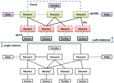
fully with the problem of model selection because competing models contribute to the overall prediction. Major research works in nonparametric Bayesian SRL approaches are NP-BLOG [Carbonetto et al., 2005], infinite (hidden) relational models [Kemp et al., 2006; Xu et al., 2006], and relational Gaussian processes [Chu et al., 2006; Yu et al., 2006; Yu and Chu, 2007; Silva et al., 2007].
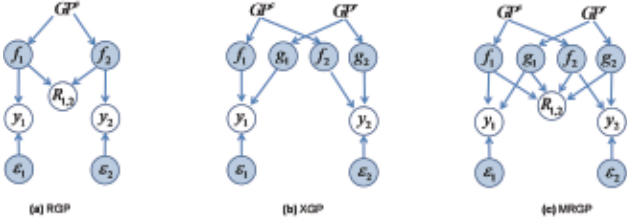
Considering the movie recommendation example, we can model it with Gaussian processes along the lines of Chu et al. [2006] based on the friend relation only. Essentially, we introduce latent variables f(xi) (shortened as fi) for the noise-free recommendations drawn from a Gaussian process for each person. xi is an attribute vector of person i. Now, we add relational information by conditioning on relational indicators such as friend. That is we let friendi,j be an indicator that assumes different values 1 or 0 depending on whether person i is a friend of j or not. Then a likelihood distribution P(friendi,j = 1|fi, fj) can be defined with a sigmoid function. It essentially encodes a constraint on fi and fj making sure that fi and fj correlate if friendi,j is true. The evidence is incorporated into the Gaussian process by conditioning on all indicators that are positive. The essential dependency structure of the probabilistic model is depicted in Fig. 2(c).
Chu et al.'s as well as other Gaussian process models only focus on one single relation between two types of entities. In this paper, we present a multi-relational Gaussian process (MRGP) model that is able to deal with an arbitrary number of relations and entity types in a domain of interest. The key idea is to introduce latent random variables gi resp. fi for all relations and entity types as depicted in Fig. 2(c). Now, we model the relational indicator friendi,j is conditioned on the linear combination of all latent variables involved in the relation. Because we condition on the indicators, the relation-wise and entity-wise Gaussian processes exchanges information between the participating GPs through the entire multi-relational network. Our experiments on real-world data demonstrate that simultaneously utilizing all relations and entity types in a domain of interest can indeed improve the quality of predictions.
The paper is organized as follows. We start off with related work. Then, we will introduce MRGPs and discuss how to model different types of relations in Sec. 3. Sec. 4 will describe approximate inference and hyperparameter estimation. Before concluding, we will present the experimental results in Sec. 5.
2 RelatedWork
There have been many research efforts in multi-relational learning [Getoor and Taskar, 2007; De Raedt, 2008]. The application of Gaussian processes [Rasmussen and Williams, 2006] to relational learning, however, has been fairly recent. Two issues need to be addressed for relational Gaussian process models: First, one needs to decide at which level the Gaussian processes are defined, and, second, one needs to decide how to incorporate the relation knowledge. One line of research [Chu et al., 2006; Yu et al., 2006; Yu and Chu, 2007] introduced GP models where the same type of entities share a common GP. For each entity i of type c, there are d latent variables associated (d = 1 in [Chu et al., 2006]), all of which are generated fromGP c . In MRGPs, as we will show in the next section, there are Gaussian processes introduced for each type of relations. Similar to MRGPs, Silva et al. [Silva et al., 2007] use a Gaussian process reserved to model the relations but here only one Gaussian process is employed. For modeling relations, there have been essentially two strategies followed in existing work. One is encoding relations in the covariance matrix [Zhu et al., 2005; Silva et al., 2007]. The other is encoding relations as random variables conditioned on the latent variables of entities involved in relations [Chu et al., 2006; Yu et al., 2006; Yu and Chu, 2007]. In MRGPs, we essentially combine the two strategies. An important property of relational system is that predicted relations depend on known relations. For example, prescribed procedures u of a patient will influence his future procedure u∗ with likelihood P(u∗|f(u)), where f(·) is a nonparameterized function of the prescribed procedures. Thus it is natural to encode relations both in the covariance matrix and as random variables. Fig. 2 illustrates the differences between these models. The linear combination of latent variables used in MRGPs is similar to Singh and Gordon's [2008] generalization of linear models to multirelational domains.
3 Multi-relational Gaussian Process Model
In this section, we will give a detailed description of the multi-relational GP (MRGP) model, and analyze it in the context of different types of relations.
3.1 Basic Idea
Reconsider our social movie recommendation scenario. Multi-relational GP models have several latent variables for each entity and several latent variables for each relation. The latent variables capture the basic information about entities and relations. Specifically, let's first consider the entities, i.e. persons and movies. To capture the basic information/profile of a person (that a priori only depends on the person's attribute) we add a variable for the person
In the example, each person can be involved in two relations: friend and like. Therefore we add
encoding the person's preference on friendships and movies. Similarly, we proceed for movies. Because movies are only involved in the like relation, we add only two latent variables, namely f m k ∼ GP(0,Σm) capturing a movie's basic profile and hlike,m k ∼ GP(0,Σlike,m) representing a movie's role in the like relation. The latent variables are coupled via the observed relations. We represent each relation as a random variable, which is a common child of all latent variables involved in the relation. Consider for example the like relation between person i and movie k. We introduce the variable Rlike i,k as a common child of f p i , f m k , hlike,p i , and hlike,m k . To represent the infinitely many values the parents can take in the conditional probability distribution, we aggregate their joint state in a variable ξ like i,k . Several aggregation function are possible. In this paper, we use a linear combination, i.e.,
where ωlike is a vector of mixing weights. Then, we set
where Φ(·) is a sigmoid function. Now, conditioning on Rlike i,k couples the relevant latent variables. Note that with the latent variable f p i representing basic profiles of entities, relations of different types are coupled together. Similarly, the class label yp i of a person i can be modeled as P(yp i |ξ p i ) = Φ(ξ p i ), where ξ p i = (f p i , hlike,p i , gfriend,p i )· ωp . In other words, persons are classified taking all (heterogeneous) information about the persons into account.
The basic idea underlying the MRGP model can also be formulated in the following way. Assume that the class label yp i of a person i is conditioned on a function value ξ p i of person attributes xi, friendships ui and favorite movies vi:
where φ(·) is a set of basis functions mapping the input vector into a higher dimensional feature space where the input vectors are (obviously) distinct. Since xi, ui and vi come from different information sources, it is natural that in different, higher dimensional feature spaces (i.e., mapping functions), the heterogeneous inputs are distinguished respectively. Thus, we introduce for each information source a distinct set of basis functions, and get a multiple GP model.
Note, that ω1, ω2 and ω3 are vectors of different dimensionality. Finally, ωp is a three dimensional weight vector, which combines the latent function values together.
3.2 The Model
The social movie recommendation example can be generalized to the general multi-relational case as summarized in Fig. 2(c):
- With each entity type c, there are multiple Gaussian processes associated: GP(0,Σc ) for entity attributes, and GP (0, Σr,c ) for each relation b in which this type of entities participate.
- For each entity i of type c:
- Add a latent variable f c i drawn fromGP(0,Σc ) encoding the essential property of the entity.
- Add a latent variable gr,c i drawn fromGP(0,Σr,c ), if the entity is involved in the relation r. It represents the hidden causes for the entity to be involved in the relation r.
- Each relation Rr i,j between entities i and j has two states, +1 if the relation is true, -1 otherwise. The likelihood is P(Rr i,j = +1|ξ r i,j ) = Φ(ξ r i,j ), where Φ(·) is a sigmoid function and ξ b i,j aggregates the involved latent variables. For simplification, we use a linear model:
where ci and cj are the types of the entities i and j, ωr = (ωr 1 , . . . , ωr 4 ) is a vector of mixing weights. Since the weights are just to scale the latent variables, we can integrate them into the parameters of covariance functions, then Eq. (1) simplifies to
Assuming finitely many entities and relations it is clear that a MRGP is well-defined, i.e., it encodes a proper probability density. Moreover, the latent variable f c i is involved in all relations the entity i appears in. Consequently different types of relations are coupled, which also motivates the name of our model: multi-relational Gaussian processes.
3.3 Types of Relations
In real-world domains, one typically encounters several types of relations: bipartite relations between different entity types, directed and undirected relations between entities of the same type. Within MRGPs, we can easily encode the different types of relations. Notice that latent variables on relations of the same type share a Gaussian process with mean function μ = E(ξ r i,j ) and covariance function k(ξ r i,j , ξ r i′ ,j ′). Without loss of generality, we assume the mean is zero. By using the right covariance function, we can encode the different types of relations as will show now.
Bipartite relations involve entities of different types, e.g., like: person × movie. The latent variable of a relation between a person i and a movie k can be written as
Intuitively, f p i and f m k respectively represent the essential profiles of the person i and the movie k, glike,p i and glike,m k respectively represent the preference of the person i on movies and the preference of the movie k on persons. Eq. (3) reveals that whether a person likes a movie is dependent on the person's profile, the movie's profile, and the person's preference on movies, as well as the movie's preference on persons. The corresponding covariance function can be written as
In directed univariate relations, the pairs of entities are of the same type but ordered. Consider e.g. citations of papers cite: paper × paper. Such relations give raise to nonsymmetric matrixes, and the entities typically play different roles such as the citing and the cited paper. The latent variable of a relation from a paper i to a paper j is written as
because the relation is univariate, f p i and f p j are drawn from the same GP. The latent variables gciting i and gcited j , however, are drawn from different GPs, since they represent the preferences of the different roles. The covariance function k(ξ cite i,j , ξ cite i′ ,j ′) can be set to
Undirected univariate relations are symmetric, i.e., there is no semantic direction. As an example consider friend: person × person. The latent variable of a relation from a person i to a person j is written as
Because the two involved entities play the same role, we do not need to distinguish them, thus gfriend,p i and gfriend,p j are drawn from the same GP. The covariance function k(ξ friend i,j , ξ friend i′ ,j ′ ) is set to
which is indeed symmetric because the following four covariances between relations Ri,j, Rj,i, Ri′ ,j ′ , Rj ′ ,i′ equal: k(ξ friend i,j , ξ friend i′ ,j ′ ), k(ξ friend i,j , ξ friend j ′ ,i′ ), k(ξ friend j,i , ξ friend i′ ,j ′ ), and k(ξ friend j,i , ξ friend j ′ ,i′ ).
3.4 The Covariance Functions
Finally, we need to define sensible covariance functions for the GPs. There are two types of covariance matrices, namely the attribute-wise ones and the relation-wise ones, which we will now discuss in turn.
The attribute-wise latent variable f c i ∼ GP(0,Σc ) represents the essential profile of an entity. In the GP framework, the covariance matrix Σc can be derived from entity attributes xci with any kernel functions k(xci , xcj ), e.g. the squared exponential covariance function.
For relation r between entity types ci and cj, there are two GPs associated, namely GP(0,Σr,ci ) for ci and GP (0, Σr,cj ) for cj . There are generally two strategies to define the covariance matrices. The simplest way is to represent the known relations of entity i as a vector. Then the relationwise covariance matrix can be computed like the attributewise ones. Alternatively, we can employ graph-based kernels, see e.g. [Zhu et al., 2005; Silva et al., 2007]. However, there is one difficulty in the multi-relational case. If the relations are bipartite, i.e., ci ̸= cj, then the graph kernels for univariate relations are not applicable. We address the problem by projecting the bipartite relations to univariate ones. Specifically, we add a relation between entities i and j iff. both entities link to the same (heterogeneous) entity. Then we can compute the graph kernels on the projected graphs. For example, we can convert a bipartite relation Direct: movie × person to an undirected one Co-Directed: movie × movie.
Finally, let us touch upon the case that attributes or relations are not informative, missing or unavailable. In this case, the covariance matrices will not be reliable and it would be better to estimate it from data. To do so, we assume the covariance matrix has an inverse Wishart distribution Σ ∼ W -1 (Σ0, β).
4 Inference and Parameter Learning
So far, we have described the MRGP model. In this section, we will discuss the inference and the hyperparameter estimation for MRGPs.
Let us illustrate the inference procedure on the movie recommendation example. Without loss of generality, we only consider the relations like. The inference involving multi-types of relations can be derived straightforwardly. Assume there are N persons, M movies and N × M ratings. The latent variables are f p = {f p 1 , . . . , f pN }, f m = {f m 1 , . . . , f m M } and glike,p = {glike,p 1 , . . . , glike,p N }, glike,m = {glike,m 1 , . . . , glike,m M }. The key inference problem is to compute the posterior over the latent variables given ratings R: P(f p , f m, glike,p , glike,m|R) ∝
where ξ is a linear combination of f p , f m, glike,p , glike,m, see Eq. (3). We assume that a rating of person i on movie k has the likelihood
Ri,k is 1 if the user likes the movie, -1 otherwise. Unfortunately, computing this posterior is intractable because P (R|ξ) is non-Gaussian, and because ξ is a weighted sum of multiple latent variables coupling the GPs. Therefore, we stick to approximate inference. To solve the computational complexity introduced by coupling of GPs, we directly compute the posterior of ξ instead of that of f p , f m, glike,p and glike,m. More precisely, we compute P (ξ|R) ∝ P (ξ)P (R|ξ) where P (ξ) is the prior of ξ, which is a GP with mean and covariance matrix as discussed in the previous section. Then, we use the expectation propagation (EP) algorithm [Minka, 2001] to approximate the posterior, i.e., we use an unnormalized Gaussian distributions ti,k(ξi,k|˜μi,k, ˜σ2 i,k , ˜ Zi,k) to approximate Eq. (10). In the inference procedure, we update the approximations for each latent variable ξi,k sequentially until convergence.
We learn the hyperparameters θ under the empirical Bayesian framework. The hyperparameters include the parameters of kernel functions and the means of the GPs. We seek θ∗ = argmaxθ logP(R|θ) =
where the prior P(ξ|θ) is a Gaussian process, but the likelihood P(R|ξ) is not Gaussian, thus the integral is analytically intractable. To solve the problem, we approximate the log likelihood with un-normalized Gaussian distributions:
-
where ˜Σ is a diagonal matrix, whose entries are ˜σ2 i,k . C can be viewed as a constant for our purpose (which can be omitted). We propose a generalized Expectation Maximum approach to learn the hyperparameters. In the E step, the EP parameters (˜μi,k, ˜σ2 i,k , ˜ Zi,k) are optimized to approximate the posterior of latent variables with the current values of hyperparameters. The approximation procedure has been discussed above. In the M step, the hyperparameters are optimized to maximize the log marginal likelihood. We omit the derivation of the gradient due to space restrictions.
5 Experimental Evaluation
To investigate the performance of the multi-relational Gaussian process model MRGPs, we empirically evaluated it in different scenarios: (1) multiple relations, (2) multiple types of entities, and (3) directed relations. To this end, we implemented the model and compared it with Silva el al.'s [2007] recent relational Gaussian process model called XGPs 1 with the default settings provided by Silva et al. For MRGPs, we maximized the likelihood as described in the previous section with the l2-norm of the weights as penalty term to prevent overfitting using SCG. In the experiments, we use the Gaussian kernel for the attribute-wise covariance function, and the graph kernel [Silva et al., 2007] for the relation-wise covariance function. The performance was evaluated with the area under the ROC curve (AUC).
5.1 Multiple Relations
Domains with multiple relations are especially interesting for evaluating the MRGP models. We perform experimental analysis with the Rummel's [1999] dataset on dimensionality of nations. The dataset includes 14 countries, 54 binary predicates representing interactions between countries, and 90 features of the countries as preprocessed by Kemp et al. [2006]. The task was to predict whether a country is a communist or not based on their attributes and relations. We selected two relations, namely conferences and time since ally. To do so, we ran XGPs on all 54 relations separately and selected the two that XGPs did not achieve an AUC score of 1.0.
We conducted the experiments with a transductive setting where both relations were used to learn MRGPs, and comparisons were made with XGPs using only one relation for predicting the labels of unlabeled samples. We randomly selected two nations, one communist and the other not, to learn the models. Then we predicted the labels of the remaining unlabeled nations. Of course, the feature "communist" was excluded from the countries' features. Table 1 summarizes the results over 10 runs. It shows that using two relations is clearly beneficial. With only one relation, MRGPs perform similar to XGPs. Combining both relations substantially increased the AUC score.
1 http://www.statslab.cam.ac.uk/ silva/code/xgp/
| XGP | MRGP | ||||
|---|---|---|---|---|---|
| R1 | R2 | R1 | R2 | R1+R2 | |
| Mean | 0.8296 | 0.8296 | 0.8370 | 0.8259 | 0.8556 |
| Var. | 0.0226 | 0.0226 | 0.0229 | 0.0189 | 0.0294 |
| 90% | 80% | 70% | 60% | ||
|---|---|---|---|---|---|
| MRGP | Mean | 0.6503 | 0.6272 | 0.6298 | 0.6236 |
| Var. | 0.0024 | 0.0006 | 0.0005 | 0.0003 | |
| IHRM | Mean | 0.6402 | 0.5681 | 0.5411 | 0.5305 |
| Var. | 0.0021 | 0.0024 | 0.0008 | 0.0006 |
5.2 Multiple Types of Entities
In contrast to XGPs, MRGPs can deal with multiple types of entities. We evaluated this feature of MRGPs with the MovieLens data [Sarwar et al., 2000]. We randomly selected a subset with 100 users, 50 movies and 1061 relations for the experiment. The task is to predict the preferences of users on the movies. The users have attributes Age, Gender, Occupation, and the movies have attributes Published-year, Genres and so on. The like relations have two states, where R = 1 indicates that the user likes the movie and -1 otherwise. Note that the user ratings in MovieLens are originally based on a five-star scale, so we transfer each rating to binary value with R = 1 if the rating is higher than the user's average rating, and vice versa. Again, the experiments are performed with the transductive-learning setting, i.e. the information about both training and test users is considered in the learning period. XGPs can neither explore the relations involving multiple types of entities, nor predict relations. RGPs focus on domains with single type of entities and undirected relations. The MovieLens data, however, contains two types of entities and bipartite relations. So we compare MRGPs with another nonparametric Bayesian relational method: infinite hidden relational models (IHRMs) [Xu et al., 2006], which introduce Dirichlet process into relational learning. We randomly select 90% (80%, 70%, 60%) ratings as known ones, and predict the remaining ones. We run the experiment 30 times and report the averaged AUC scores of rating predictions. As shown in the experimental results in Table 2, MRGPs display better performance than IHRMs.
5.3 Directed Relations
The presence of directed relations over entities of the same type is also an interesting scenario for MRGPs. We perform experimental analysis with the same subset of the WebKB dataset as in the work of Silva et al. [2007]. The subset contains 4160 pages and 9998 hyperlinks interconnecting them from 4 different universities, as well as features describing the content of the web pages. In contrast to the work of Silva et al., we use the directed link relations. We compared MRGPs with XGPs on the performance of predicting if a webpage is of class "other" or not. We used the first 20 subsamples, where 10% of the whole data is sampled from the pool for a specific university, and the remaining is used for test. We also used the same webpage features as Silva et al. The results show that MRGPs perform similar to XGPs. For instance, the mean and standard deviation of AUC in the Cornell University results were 0.934 ± 0.037 for MRGPs and 0.917 ± 0.022 for XGPs. In the results of the University of Washington, they were 0.923 ± 0.02 for MRGPs and 0.923 ± 0.016 for XGPs. XGPs convert the directed links into two undirected links, and manually selects the one with better performance. Whereas MRGPs can model direction of relations, and executes the selection procedure implicitly and automatically.
We have evaluated MRGPs with three categories of relational data. To summarize, the experimental results showed that exploiting the correlations among different entity types and relations can indeed improve the prediction performance.
6 Conclusion
In this paper we proposed a nonparametric Bayesian framework for multi-relational data. The resulting multi-relational Gaussian process (MRGP) model combines the covariance and the random variables approaches to model multiple relations within Gaussian processes. It provides a flexible tool for many relational learning tasks with multiple types of entities and relations. The experimental results on several real-world datasets show a performance gain of multiplerelational Gaussian processes over single relational ones.
MRGPs suggest several interesting directions for future research such as sparse MRGPs, developing multi-relational variants of dimensionality reduction techniques [Lawrence, 2005] and of ranking techniques [Guiver and Snelson, 2008], and applying MRGPs in spatial-relational domains such as computer vision and robotics.
7 Acknowledgments
The authors would like to thank the anonymous reviewers for their comments. This research was supported by the Fraunhofer ATTRACT fellowship STREAM, the German Federal Ministry of Economy and Technology (BMWi) research program THESEUS, and the EU FP7 project LarKC.
@inproceedings{ijcai2009p220,
  title     = {Multi-Relational Learning with Gaussian Processes},
  author    = {Xu, Zhao and Kersting, Kristian and Tresp, Volker},
  booktitle = {Proceedings of the Twenty-First International Joint Conference on
               Artificial Intelligence, {IJCAI-09}},
  publisher = {International Joint Conferences on Artificial Intelligence},
  editor    = {Craig Boutilier},
  pages     = {1309--1313},
  year      = {2009},
  url       = {https://ijcai.org/proceedings/2009/220},
}
TY - CPAPER TI - Multi-Relational Learning with Gaussian Processes AU - Xu, Zhao AU - Kersting, Kristian AU - Tresp, Volker T2 - Proceedings of the Twenty-First International Joint Conference on Artificial Intelligence, IJCAI-09 PB - International Joint Conferences on Artificial Intelligence PY - 2009 SP - 1309 EP - 1313 UR - https://ijcai.org/proceedings/2009/220 ER -Copied
Machine-readable versions of this paper, for tools and AI agents:





