
Preference Learning with Extreme Examples
Proceedings of the Twenty-First International Joint Conference on Artificial Intelligence. Pages 1285-1289.
© 2009 International Joint Conferences on Artificial Intelligence
Abstract
In this paper, we consider a general problem of semi-supervised preference learning, in which we assume that we have the information of the extreme cases and some ordered constraints, our goal is to learn the unknown preferences of the other places. Taking the potential housing place selection problem as an example, we have many candidate places together with their associated information (e.g., position, environment), and we know some extreme examples (i.e., several places are perfect for building a house, and several places are the worst that cannot build a house there), and we know some partially ordered constraints (i.e., for two places, which place is better), then how can we judge the preference of one potential place whose preference is unknown beforehand? We propose a Bayesian framework based on Gaussian process to tackle this problem, from which we not only solve for the unknown preferences, but also the hyperparameters contained in our model.Fei Wang, Bin Zhang, Ta-Hsin Li, Wenjun Yin, Jin Dong, Tao Li
- [Agarwal et al., 2006] A. Agarwal, S. Chakrabarti, and S. Aggarwal. Learning to rank networked entities. In The 12th ACM SIGKDD international conference on Knowl- edge discovery and data mining, pages 14-23, 2006.
- [Bahamonde et al., 2004] A. Bahamonde, G. Bayón, J. Díez, J. Quevedo, del Coz., J. Alonso, and F. Goyache. Fea- ture subset selection for learning preferences: a case study. pages 49-56, 2004.
- [Belkin et al., 2006] M. Belkin, P. Niyogi, and V. Sindhwani. Manifold regularization: a geometric framework for learn- ing from labeled and unlabeled examples. Journal of Ma- chine Learning Research, 7:2399-2434, 2006.
- [Chapelle et al., 2006] O. Chapelle, B. Schölkopf, and A. Zien. Semi-supervised learning. MIT Press, 2006.
- [Chu and Ghahramani, 2004] W. Chu and Z. Ghahramani. Gaussian processes for ordinal regression. Journal of Ma- chine Learning Research, 6:2005, 2004.
- [Chu and Ghahramani, 2005] W. Chu and Z. Ghahramani. Preference learning with gaussian process. In The 22nd In- ternational Conference on Machine Learning, pages 137- 144, 2005.
- [Chu and Keerthi, 2007] W Chu and S Keerthi. Support vec- tor ordinal regression. Neural Computation, 19(3):792- 815, 2007.
- [Doyle, 2004] D. Doyle. Prospects of preferences. Compu- tational Intelligence, 20:111-136, 2004.
- [Herbrich et al., 1998] R. Herbrich, T. Graepel, P. Bollmann, Sdorra, and K. Obermayer. Learning a preference relation in ir. In Proceedings Workshop Text Categorization and Machine Learning, International Conference on Machine Learning, pages 80-84, 1998.
- [Kapoor et al., 2005] A. Kapoor, Y. Qi, H. Ahn, and R. W. Picard. Hyperparameter and kernel learning for graph based semi-supervised classification. In Advances in Neu- ral Information Processing Systems, pages 627-634, 2005.
- [Kim and Ghahramani, 2006] H.-C. Kim and Z. Ghahra- mani. Bayesian gaussian process classification with the em-ep algorithm. Pattern Analysis and Machine Intelli- gence, IEEE Transactions on, 28(12):1948-1959, 2006.
- [Minka, 2001] T. Minka. Expectation propagation for ap- proximate bayesian inference. In Proceedings of the 17th Uncertainties in Artificial Intelligence, pages 362-369, 2001.
- [Nuray and Can, 2003] R. Nuray and F. Can. Automatic ranking of retrieval systems in imperfect environments. In The 26th annual international ACM SIGIR conference on Research and development in informaion retrieval, pages 379-380, 2003.
- [Shashua and Levin, 2003] A. Shashua and A. Levin. Rank- ing with large margin principle: Two approaches. In Advances in Neural Information Processing Systems 14, 2003.
- [Xi et al., 2004] W. Xi, J. Lind, and E. Brill. Learning effec- tive ranking functions for newsgroup search. In The 27th annual international ACM SIGIR conference on Research and development in information retrieval, pages 394-401, 2004.
- [Yu, 2005] H. Yu. Svm selective sampling for ranking with application to data retrieval. In The 11th ACM SIGKDD international conference on Knowledge discovery in data mining, pages 354-363, 2005.
- [Zheng et al., 2007] Z. Zheng, K. Chen, G. Sun, and H. Zha. A regression framework for learning ranking functions us- ing relative relevance judgments. In The 30th annual in- ternational ACM SIGIR conference on Research and de- velopment in information retrieval, pages 287-294, 2007.
- [Zhou et al., 2004] D. Zhou, J. Weston, A. Gretton, O. Bous- quet, and B. Schölkopf. Ranking on data manifolds. Advances in Neural Information Processing Systems 16, pages 169-176, 2004.
- [Zhu, 2005] X. Zhu. Semi-Supervised Learning with Graphs. PhD thesis, Carnegie Mellon University, 2005.
References were extracted automatically from the PDF and may contain errors.
Full text extracted automatically from the PDF; figures, tables and equations may differ. The PDF is the version of record.
1 Introduction
The problem of finding out the preferences of an individual exists in many real world applications. For example, a real estate developer evaluating the potential housing places, a customer judges the value of a book, a user assess his/her interests to a movie. Clearly, evaluating the preferences of all the individuals is quite time consuming and almost impossible. Therefore the development of automatic preference prediction (or preference learning) algorithms is an important and valuable research topic.
In recent years, many preference learning algorithms have been emerged in artificial intelligence [Doyle, 2004], machine learning [Bahamonde et al., 2004][Chu and Ghahramani, 2005][Chu and Keerthi, 2007], data mining [Agarwal et al., 2006][Yu, 2005] and information retrieval [Herbrich et al., 1998][Nuray and Can, 2003][Xi et al., 2004][Zheng et al., 2007] fields. Most of these algorithms takes preference learning as a supervised learning problem, i.e., we are given a set of instances {xi}ni=1 which are associated with a partial or complete order relation. Our goal is to learn a "ranking function" from whose data such that it can predict the ranks of new testing instances. However, those type of methods usually suffer from two main problems:
∗The work of F. Wang and T. Li is supported by NSF grants IIS0546280, DMS-0844513 and CCF-0830659.
- Generally training a model in a supervised way needs a large amount of "labeled" data (i.e. the data with known orders or preferences). However, in most of the real world cases, we may only known partial order information contained in the data set.
- There are usually some free parameters contained in the preference prediction model. How to tune those parameters automatically is a headache for most of the algorithms. Generally these parameters are set empirically.
Based on the above considerations, in this paper, we investigate a novel problem called semi-supervised preference learning (SSPL). In SSPL, we use both labeled (or ordered) data and unlabeled (or unordered) data to train a preference prediction model, that is because in most of the cases, unlabeled data is far easier to obtain (e.g., by crawling the web). These unlabeled data are invaluable resources and how to use them to aid the classification (or regression) task has widely been researched in semi-supervised learning field [Chapelle et al., 2006], but the similar problem in preference learning has rarely been touched. In SSPL, we consider the following two types of supervised information
- Partially ordered information. This type of information the same as in traditional preference learning algorithms. We assume that we know some ordered information on a small portion of data items.
- Extreme preferences. We also suppose that we know some preference information on the extreme cases (i.e., the cases are extremely preferred or disliked by the user, that is, the cases with the highest and lowest preference scores). This type of information is also easy to obtain in many applications. To demonstrate the effectiveness of this type of information, we give an illustrative example in Fig.1.
By incorporating those supervised information, we propose a Bayesian probabilistic kernel approach for preference learning using Gaussian process in this paper. We impose a Gaussian process prior distribution on the latent preference prediction function, and employ an appropriate likelihood function which is composed of two parts: one is a Gaussian function which measures the prediction loss on extreme preferences; the other is a generalized probit function measuring the consistency of the predicted preferences and the known ordered information. Moreover, the expectation propagation (EP) technique [Minka, 2001] is adopted to automatically tune the hyperparameters contained in the model. Finally we apply our method to a practical housing potential application problem which demonstrates the effectiveness of our method.
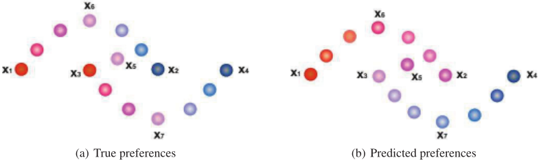
It is worthwhile to highlight several aspects of the proposed approach here:
- Our model is a semi-supervised model, which can make use of more information compared to traditional supervised model. Moreover, the supervised model can be regarded as a special case of our semi-supervised model with all the data items having their relevant supervised information.
- Unlike in traditional supervised models where we need to set the model parameters empirically, the model parameters can be self-adapted in our approach.
- Unlike some traditional semi-supervised approach (e.g., [Zhou et al., 2004]) which can only predict the preference of those "unlabeled" data, our method can be easily extended to predict the preferences of new testing data items.
The rest of this paper is organized as follows. In section 2 we will introduce our Bayesian inference framework in detail, the experimental results on benchmark data sets will be introduced in section 3. In section 4 we will introduce the background of a real world housing potential application problem, and show the detailed procedure of how to apply our model to solve the problem, and demonstrate the results, followed by the conclusions in section 5.
2 Semi-supervised Preference Learning Under a Bayesian Framework
Consider a set X of n distinct data items xi ∈ Rd , in which XL = {xi}li=1 are the extreme cases and we know their associated preferences in prior. Besides, we also have a set of observed pairwise preference relations on data items E = {(xu, xv)}, such that if (xu, xv) ∈ E, then f(xu) ≤ f(xv), which means that data item xu is less preferred than xv, and f is the latent preference prediction function. For example, in the housing potential place selection problem, f(xu) ≤ f(xv) means it is more appropriate to build a house on place xv than place xu.
Let O be the observations including XL and E, then the posterior of the latent preference function vector f = [f(x1), f(x2), · · · , f(xn)]⊤ given the observation O is
The term, p(f ) is the prior. It enforces a smoothness constraint and depends upon the underlying data manifold. Similar to the spirit of graph regularization [Zhu, 2005][Zhou et al., 2004], we use similarity graphs and their transformed Laplacian to induce priors on the preferences f . The second and third term, p(XL|f ) and p(E|f ) are the likelihoods that incorporate the prior information provided by the extreme examples and the data in E.
2.1 Gaussian Process Prior
The latent function values f(xi) are assumed to be a realization of random variables in a zero-mean Gaussian Process, then this Gaussian process can be fully specified by the covariance matrix. To define a proper covariance matrix, we recall a basic principle in graph based methods [Zhu, 2005]: the predicted data labels should be sufficiently smooth with respect to the data graph. The smoothness of f with respect to the data graph could be measured by
where Kij is the value of the (i, j)-th element in the data kernel matrix K ∈ Rn×n, L = I -D-1/2KD-1/2 ∈ Rn×n is the normalized graph Laplacian [Zhou et al., 2004]. D is the diagonal degree matrix with the i-th element on its diagonal line dii = ∑j Kij . Then we can construct a data dependent prior distribution of f as
where ˜L = L + ζI is the diagonal-jittered Laplacian matrix which is positive definite with some constant ζ [Kapoor et al., 2005], Zf is normalizing constant which makes P(f ) a probability distribution. Such a prior in fact encodes some geometrical information of data distribution P(x) [Belkin et al., 2006], e.g. if two data items xi and xj are close in the intrinsic geometry of P(x), then the conditional distributions of P (fi|xi) and P (fj |xj ) should be similar, where fi denotes the preference of xi.
2.2 Likelihood
The likelihood of the observations O = {XL, E} given the latent function f should be composed of two parts, one part measures the loss between the predictions and the actual preferences (denoted by {yi}) of XL, the other measures the loss between the predictions and E. The loss between f(xi) and yi can be simply computed by a square function, therefore the likelihood of {yi} given f can be evaluated as
Following [Chu and Ghahramani, 2005], the ideal noisefree case for the likelihood of (u, v) ∈ E is
In real world case, the preferences are usually contaminated by some noise. If we assume such noise are a zero mean Gaussians, then
where zk = fvk -fuk √2ρ , and Φ(z) = ∫ z-∞ N(δ; 0, 1)dδ. Note that we use k to denote the entry index in E. Then the total likelihood of E given f becomes
Therefore the total likelihood of the observations O given f becomes
2.3 Approximate Inference
In this paper, we use Expectation Propagation (EP) to obtain a Gaussian approximation of the posterior P (f |O). Although, the prior derived in section 2.1 is a Gaussian distribution, the exact posterior is not a Gaussian due to the form of the likelihood. We use EP to approximate the posterior as a Gaussian. EP has been previously used [3] to train a Bayes Point Machine, where EP starts with a Gaussian prior over the classifiers and produces a Gaussian posterior. Our task is very similar and we use the same algorithm. In our case, EP starts with the prior defined in Eq.(3) and incorporates likelihood to approximate the posterior P (f |O, X ) ∼ N (¯f , Σf ), where N denotes a normal distribution.
2.4 Hyperparameter Learning
We apply an EM-EP style algorithm [Kim and Ghahramani, 2006] to estimate the hyperparameters in our algorithm, which is also referred to as evidence maximization [Kapoor et al., 2005]. Denote the parameters of the kernel as ΘK, then the parameters contained in our algorithm are Θ = {ΘK, ζ, ρ}. Under the EM-EP framework, in the E-step of the EM algorithm, we use EP to approximate the posterior q(f ); in the M-step, we maximize the following lower bound according to the Jensen's inequality
The EM procedure alternates between the E-step and the M-step until convergence.
- E-Step. Given the current parameters Θi , approximate the posterior q(f ) ∼ N (¯f , Σf ) by EP.
- M-Step. Update
In the M-step the maximization with respect to the Θ cannot be computed in a closed form, but can be solved using gradient descent. The gradients of the lower bound with respect to the parameters are as follows:
where in the last equation, fk = [fvk , fuk ]⊤, a = [-1, 1]⊤, μk = Bk ¯f , and Σk = BkΣfB⊤k and Bk = [e⊤uk , e⊤vk ]⊤ ∈ R2×n and euk , evk ∈ R1×n are indicator vectors for uk and vk with all their elements being 0 except for the uk-th (or vkth) element being 1. This complicated integration can be approximated by Gaussian quadrature or Romberg integration at some appropriate accuracy.
2.5 Induction for Out-of-Sample Data
We denote the optimal parameter setting inferred from the EM-EP procedure to be Θ∗ . For a new coming case x, its latent preference value fx together with the latent preference vector f ∈ Rn×1 of the training samples follows a joint multivariate Gaussian prior, i.e.,
where k = [k(x, x1), k(x, x2), · · · , k(x, xn)]⊤ and k(·, ·) is some pre-defined kernel function, where Σ = ˜L-1 . The conditional distribution of fx given f is also a Gaussian, denoted as P (fx|f , Θ∗ ), with mean f ⊤Σ-1k and variance k(x, x) - k⊤Σ-1k. The predictive distribution of P (fx|O, X , Θ∗ ) can be computed as an integral over the f-space, i.e.,
where P(f|O,X,Θ∗ ) is a Gaussian posterior distribution of f approximated by the EM-EP procedure, then the predictive distribution (14) can be simplified as a Gaussian N (fx; μx, σ2x) with
3 Experiments on Benchmark Data Sets
In this section, we will present the results of applying our algorithm to several benchmark data sets.
3.1 Data Sets
We test the performance of our algorithm on five benchmark data sets downloaded from http://www.liacc.up. pt/˜ltorgo/Regression/DataSets.html, whose target values were discretized into ordinal quantities using equal-length binning. These bins divide the range of target values into a given number of intervals that are of same length. The resulting rank values are ordered, representing these intervals of the original metric quantities. Table 1 summarizes the basic characteristics of those data sets, where "Size" denotes the number of instances in the data set; "Dimension" indicates the dimensionality of the data points; "# Training" is the number of instances used for training; "# Testing" is the number of instances used for testing.
3.2 Methods for Comparison
Beside our method, we also implemented some other competitive methods for comparison including
| Data Sets | Size | Dimension | # Training | # Testing |
|---|---|---|---|---|
| Diabetes | 2 | 43 | 30 | 13 |
| BreastCancer | 32 | 194 | 130 | 64 |
| Pyrimidines | 74 | 27 | 50 | 24 |
| Trizazines | 186 | 60 | 100 | 86 |
| MachineCPU | 209 | 6 | 150 | 59 |
| BostonHouse | 506 | 13 | 300 | 206 |
- SVM. This is a support vector method for ranking [Shashua and Levin, 2003]. 5-fold cross validation was used to determine the optimal values of model parameters (including the width of the Gaussian kernel and the regularization parameter), and the test error was obtained using the optimal model parameters for each formulation. The initial search was done on a 7 × 7 coarse grid linearly spaced by 1.0 in the region {(log10 C, log10 σ)| - 2 ≤ log10 ≤ 4, -3 ≤ log10 σ ≤ 3}, followed by a fine search on a 9 × 9 uniform grid linearly spaced by 0.2 in the (log10 C, log10 σ) space.
- GPPL. This is the Gaussian process preference learning (GPPL) method in [Chu and Ghahramani, 2005]. The implementation is based on the code http://www. gatsby.ucl.ac.uk/˜chuwei/plgp.htm, where gradient methods have been employed to maximize the approximated evidence for model adaptation with the initial values of the Gaussian kernel width κ and the noise ρ to be 1 and 1/d, d is the data dimensionality.
- GPOR. This is the Gaussian process ordinal regression method implemented using the EP algorithm as in [Chu and Ghahramani, 2004]. The implementation code is downloaded from http://www.gatsby.ucl.ac. uk/˜chuwei/ordinalregression.html.
- SVOR. This is the support vector ordinal regression method implemented the same as in [Chu and Keerthi, 2007], where we use implicit constraints and the code is downloaded from http://www.gatsby.ucl.ac. uk/˜chuwei/svor.htm.
For the GPPL method, we generate all the pairwise constraints from the training data, and for our semi-supervised preference learning (SSPL) method, we further provide the preferences of the extreme cases in the training set. The experimental results, including the mean absolute error and standard deviation, over 20 independent runs are summarized in Table 2. From the table we can clearly see the advantage of our method.
4 Application in Housing Potential Selection
In this section, we present a novel application of our algorithm in computer aided housing potential estimation and location recommendation system. Such an application is important since nowadays, facilities or outlets (e.g. bank branches, retail stores, automobile dealers, etc) are crucial for people's daily lives. However, it is usually expensive and time consuming for a company to evaluate the suitability of the facility site locations and optimize the site network to serve more customers. The most commonly adopted method is to hire or ask for the business consultants to write some evaluation reports on estimating whether there is big value at a location for housing. Generally consultants should investigate several factors around the housing location within a million square meters including (but not limited to)
| SVM | GPPL | GPOR | SVOR | SSPL | |
|---|---|---|---|---|---|
| Diabetes | 0.7462±0.1414 | 0.6763±0.1508 | 0.6654±0.1373 | 0.6658±0.1439 | 0.6318±0.1247 |
| Breast Cancer | 1.0031±0.0727 | 1.0055±0.0868 | 1.0141±0.0932 | 1.1243±0.1077 | 0.8796±0.0754 |
| Pyrimidines | 0.4500±0.1136 | 0.4096±0.1206 | 0.3917±0.0745 | 0.6945±0.2032 | 0.3544±0.1420 |
| Triazines | 0.6977±0.0259 | 0.6783±0.0198 | 0.6878±0.0295 | 0.7033±0.0276 | 0.6248±0.0193 |
| MachineCPU | 0.1915±0.0423 | 0.1793±0.0562 | 0.1856±0.0424 | 0.2136±0.1033 | 0.1536±0.0317 |
| Boston House | 0.2672±0.0190 | 0.2763±0.0314 | 0.2585±0.0200 | 0.2887±0.0198 | 0.1934±0.0156 |
- The commercial services sites such as shopping centers, banks, supermarkets, carnies, amusement parks, etc.
- The social service sites such as hospitals, hotels, kindergartens, schools, colleges, etc.
- The traffic conveniences such as bus and subway stations, or even the railway and air stations.
- Other facilities such as bars and restaurants.
As an example, we show a map of housing locations along with their impact factors in Fig. 2, where different symbols represent different factors. In the figure there are totally 47 housing potential locations plotted.
After collecting all the relevant information above, the consultants need to integrate them together by assigning different weights to different factors and finally give a overall estimation of the suitability of a place. However, this may not be a good strategy since (1) the number of factors that may affect the suitability of a place could be very large, which makes the determination of their weights a hard and time consuming task; (2) the weights are usually determined manually by the consultants according to their professional experience. Therefore the construction of a mathematical model for evaluating the suitability of each location automatically is a problem worthy of researching due to its practical requirements.
Unfortunately, it is difficult to construct a good location evaluation model because
- We usually do not know the exact mechanism of evaluating those locations. As stated before, in most cases we should consider multiple factors simultaneously to evaluate whether a location is good or bad, e.g., in banking, we should consider deposit, loan, financial service revenue, cost, etc. Since different factors have different descriptions and scales, it is difficult to model those factors into a single objective function to be optimized.
- We usually do not have enough historical rating data of evaluating the housing locations, which makes training a proper model for evaluating new places very hard and unreliable.
Based on the above considerations, the model proposed in this paper could be very suitable for solving the housing location evaluation problem since (1) Usually the information of extreme cases are easy to obtain since the extremely good or bad locations are treated as examples to guide the consultants for their evaluations; (2) Our model need not to know the exact preferences (ratings) of each location, but only the ordered relationships between some of the pairwise locations, which is much easier to work out by consulting some experts; (3) Our model is semi-supervised, which means that we need not to collect a large amount of historical rating data, generally a small portion of them is enough; (4) Our model can tune the model parameters adaptively according to the data distributions, so the users need not to worry about how to set the optimal parameters related to different factors.
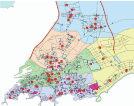
In our experiments, we just adopted the housing location distribution map shown in Fig.2 as our data set. Therefore there are totally 49 potential housing locations. For each location, we construct a 32 dimensional vector which can summarize the factors that may affect the final evaluation of the suitability of itself 1 . We label four locations as extremely good places for housing and four locations as extremely bad places for housing. For the other 41 locations, we randomly generate 20 pairwise ordered constraints, and this process is repeated 20 times. To demonstrate the superiority of our method, we also conducted two competitive approaches:
1 The vector is summarized in the following way. We first extract 32 factors (facilities) which may affect the final suitability evaluations of the housing potential locations. For each vector, the value on one dimension is the number of its corresponding facility.
| SSDML | GPPL | BSSPL | |
|---|---|---|---|
| AUROC | 0.7805 | 0.7934 | 0.8336 |
| AUROCCH | 0.8326 | 0.8533 | 0.8848 |
- The semi-supervised distance metric learning (SSDML) method [20], which does not make use of the ordered constraints.
- The Gaussian process preference learning (GPPL) method [Chu and Ghahramani, 2005], which cannot take the information on extreme cases into account.
Finally, to compare the performances of those different algorithms, we use the areas under the receiver operating characteristic ROC curve (AUROC) and convex hull of ROC curve (AUROCCH) as our criterions 2 . The final results are summarized in Table 3 (note that all the values in the table are averaged over 20 independent runs), from which we can clearly observe that our method can perform significantly better than the other two methods for this task.
5 Conclusions
In this paper, we propose a novel semi-supervised preference learning method using Gaussian process, where we assume that we are given a set of pairwise ordered constraints together with some extreme examples. We propose an EM-EP algorithm to learn the hyperparameters in our algorithm. Finally the experimental results on both benchmark data sets and real world housing potential place estimation are presented to show the effectiveness of our method.
@inproceedings{ijcai2009p216,
  title     = {Preference Learning with Extreme Examples},
  author    = {Wang, Fei and Zhang, Bin and Li, Ta-Hsin and Yin, Wen Jun and Dong, Jin and Li, Tao},
  booktitle = {Proceedings of the Twenty-First International Joint Conference on
               Artificial Intelligence, {IJCAI-09}},
  publisher = {International Joint Conferences on Artificial Intelligence},
  editor    = {Craig Boutilier},
  pages     = {1285--1289},
  year      = {2009},
  url       = {https://ijcai.org/proceedings/2009/216},
}
TY - CPAPER TI - Preference Learning with Extreme Examples AU - Wang, Fei AU - Zhang, Bin AU - Li, Ta-Hsin AU - Yin, Wen Jun AU - Dong, Jin AU - Li, Tao T2 - Proceedings of the Twenty-First International Joint Conference on Artificial Intelligence, IJCAI-09 PB - International Joint Conferences on Artificial Intelligence PY - 2009 SP - 1285 EP - 1289 UR - https://ijcai.org/proceedings/2009/216 ER -Copied
Machine-readable versions of this paper, for tools and AI agents:





