
On the Equivalence between Canonical Correlation Analysis and Orthonormalized Partial Least Squares
Proceedings of the Twenty-First International Joint Conference on Artificial Intelligence. Pages 1230-1234.
© 2009 International Joint Conferences on Artificial Intelligence
Abstract
Canonical correlation analysis (CCA) and partial least squares (PLS) are well-known techniques for feature extraction from two sets of multi-dimensional variables. The fundamental difference between CCA and PLS is that CCA maximizes the correlation while PLS maximizes the covariance. Although both CCA and PLS have been applied successfully in various applications, the intrinsic relationship between them remains unclear. In this paper, we attempt to address this issue by showing the equivalence relationship between CCA and orthonormalized partial least squares (OPLS), a variant of PLS. We further extend the equivalence relationship to the case when regularization is employed for both sets of variables. In addition, we show that the CCA projection for one set of variables is independent of the regularization on the other set of variables. We have performed experimental studies using both synthetic and real data sets and our results confirm the established equivalence relationship. The presented analysis provides novel insights into the connection between these two existing algorithms as well as the effect of the regularization.Liang Sun, Shuiwang Ji, Shipeng Yu, Jieping Ye
- [Arenas-Garcia and Camps-Valls, 2008] J. Arenas-Garcia and G. Camps-Valls. Efficient kernel orthonormalized PLS for remote sensing applications. Geoscience and Remote Sensing, IEEE Transactions on, 46(10):2872-2881, 2008.
- [Bach and Jordan, 2003] F. R. Bach and M. I. Jordan. Kernel in- dependent component analysis. Journal of Machine Learning Research, 3:1-48, 2003.
- [Barker and Rayens, 2003] M. Barker and W. Rayens. Partial least squares for discrimination. Journal of Chemometrics, 17(3):166- 173, 2003.
- [Golub and Loan, 1996] G. H. Golub and C. F. Van Loan. Matrix computations. Johns Hopkins Press, Baltimore, MD, 1996.
- [Hardoon and Shawe-Taylor, 2003] D. R. Hardoon and J. Shawe- Taylor. KCCA for different level precision in content-based im- age retrieval. In Third International Workshop on Content-Based Multimedia Indexing, 2003.
- [Hardoon et al., 2004] D. R. Hardoon, S. Szedmak, and J. Shawe- taylor. Canonical correlation analysis: An overview with appli- cation to learning methods. Neural Comput., 16(12):2639-2664, 2004.
- [Hardoon, 2006] D. R. Hardoon. Semantic models for machine learning. PhD thesis, University of Southampton, 2006.
- [Hotelling, 1936] H. Hotelling. Relations between two sets of vari- ables. Biometrika, 28:312-377, 1936.
- [Rosipal and Krämer, 2006] R. Rosipal and N. Krämer. Overview and recent advances in partial least squares. In Subspace, La- tent Structure and Feature Selection Techniques, Lecture Notes in Computer Science, pages 34-51. Springer, 2006.
- [Schölkopf and Smola, 2002] B. Schölkopf and A. J. Smola. Learning with kernels: support vector machines, regularization, optimization, and beyond. MIT Press, Cambridge, MA, 2002.
- [Shawe-Taylor and Cristianini, 2004] J. Shawe-Taylor and N. Cris- tianini. Kernel methods for pattern analysis. Cambridge Univer- sity Press, New York, NY, 2004.
- [Sun et al., 2008] L. Sun, S. Ji, and J. Ye. A least squares formu- lation for canonical correlation analysis. In ICML, pages 1024- 1031, 2008.
- [Vert and Kanehisa, 2003] J.-P. Vert and M. Kanehisa. Graph- driven feature extraction from microarray data using diffusion kernels and kernel cca. In NIPS 15, pages 1425-1432, 2003.
- [Wold and et al., 1984] S. Wold and et al. Chemometrics, mathe- matics and statistics in chemistry. Reidel Publishing Company, Dordrecht, Holland, 1984.
- [Worsley et al., 1997] K. Worsley, J.-B. Poline, K. J. Friston, and A.C. Evans. Characterizing the response of PET and fMRI data using multivariate linear models. Neuroimage, 6(4):305-319, 1997.
References were extracted automatically from the PDF and may contain errors.
Full text extracted automatically from the PDF; figures, tables and equations may differ. The PDF is the version of record.
1 Introduction
Canonical correlation analysis (CCA) [Hotelling, 1936] is commonly used for finding the correlations between two sets of multi-dimensional variables. CCA seeks a pair of linear transformations, one for each set of variables, such that the data are maximally correlated in the transformed space. As a result, it can extract the intrinsic representation of the data by integrating two views of the same set of objects. Indeed, CCA has been applied successfully in various applications [Hardoon et al., 2004; Vert and Kanehisa, 2003], including regression, discrimination, and dimensionality reduction.
Partial least squares (PLS) [Wold and et al., 1984] is a family of methods for modeling relations between two sets of variables. It has been a popular tool for regression and classification as well as dimensionality reduction [Rosipal and Kr¨amer, 2006; Barker and Rayens, 2003], especially in the field of chemometrics. It has been shown to be useful in situations where the number of observed variables (or the dimensionality) is much larger than the number of observations. In its general form, PLS creates orthogonal score vectors (also called latent vectors or components) by maximizing the covariance between different sets of variables. Among the many variants of PLS, the orthonormalized PLS (OPLS) [Worsley et al., 1997; Arenas-Garcia and Camps-Valls, 2008], a popular variant of PLS, is studied in this paper.
In essence, CCA finds the directions of maximum correlation while PLS finds the directions of maximum covariance. Covariance and correlation are two different statistical measures for quantifying how variables covary. It has been shown that there is a close connection between PLS and CCA in discrimination [Barker and Rayens, 2003]. In [Hardoon, 2006] and [Rosipal and Kr¨amer, 2006], a unified framework for PLS and CCA is developed, and CCA and OPLS can be considered as special cases of the unified framework by choosing different values of regularization parameters. However, the intrinsic equivalence relationship between CCA and OPLS has not been studied yet.
In practice, regularization is commonly employed to penalize the complexity of a learning model and control overfitting. It has been applied in various machine learning algorithms such as support vector machines (SVM). The use of regularization in CCA has a statistical interpretation [Bach and Jordan, 2003]. In general, regularization is enforced for both sets of multi-dimensional variables in CCA, as it is generally believed that the CCA solution is dependent on the regularization on both variables.
In this paper, we study two fundamentally important problems regarding CCA and OPLS: (1) What is the intrinsic relationship between CCA and OPLS? (2) How does the regularization affect CCA and OPLS as well as their relationship? In particular, we formally establish the equivalence relationship between CCA and OPLS. We show that the difference between the CCA solution and the OPLS solution is a mere orthogonal transformation. Unlike the discussion in [Barker and Rayens, 2003] which focuses on discrimination only, our results can be applied for regression and discrimination as well as dimensionality reduction. We further extend the equivalence relationship to the case when regularization is applied for both sets of variables. In addition, we show that the CCA projection for one set of variables is independent of the regularization on the other set of variables, elucidating the effect of regularization in CCA. We have performed experimental studies using both synthetic and real data sets. Our experimental results are consistent with the established theoretical results.
Notations
Throughout this paper the data matrices of the two views are denoted as X = [x1, · · · , xn] ∈ Rd1×n and Y = [y1, · · · , yn] ∈ Rd2×n, respectively, where n is the number of training samples, d1 and d2 are the data dimensionality correspond to X and Y , respectively. We assume that both X and Y are centered in terms of columns, i.e., ∑ni=1 xi = 0 and ∑ni=1 yi = 0. I denotes the identity matrix, and A† is the pseudo-inverse of matrix A.
2 Background
2.1 Canonical Correlation Analysis
In canonical correlation analysis (CCA) two different representations of the same set of objects are given, and a projection is computed for each representation such that they are maximally correlated in the dimensionality-reduced space. In particular, CCA computes two projection vectors, wx ∈ Rd1 and wy ∈ Rd2 , such that the correlation coefficient
is maximized. Multiple projections of CCA can be computed simultaneously by solving the following problem:
where each column of Wx ∈ Rd1×ℓ and Wy ∈ Rd2×ℓ corresponds to a projection vector and ℓ is the number of projection vectors computed. Assume that Y Y T is nonsingular. The projection Wx is given by the ℓ principal eigenvectors of the following generalized eigenvalue problem:
where η is the corresponding eigenvalue.
In regularized CCA (rCCA), a regularization term is added to each view to stabilize the solution, leading to the following generalized eigenvalue problem [Hardoon et al., 2004; Shawe-Taylor and Cristianini, 2004]:
where λx > 0 and λy > 0 are the two regularization parameters.
2.2 Orthonormalized Partial Least Squares
While CCA maximizes the correlation of data in the dimensionality-reduced space, partial least squares (PLS) maximizes their covariance [Barker and Rayens, 2003; Rosipal and Kr¨amer, 2006]. In this paper, we consider orthonormalized PLS (OPLS) [Worsley et al., 1997], which does not consider the variance of one of the two views. It has been shown to be competitive with other PLS variants [Worsley et al., 1997; Arenas-Garcia and Camps-Valls, 2008]. OPLS computes the orthogonal score vectors for X by solving the following optimization problem:
It can be shown that the columns of the optimal W are given by the ℓ principal eigenvectors of the following generalized eigenvalue problem:
It follows from the discussion above that the computation of the projection of X in OPLS is directed by the information encoded in Y . Such formulation is especially attractive in the supervised learning context in which the data are projected onto a low-dimensional subspace directed by the label information encoded in Y . Thus, OPLS can be applied for supervised dimensionality reduction.
Similar to CCA, we can derive regularized OPLS (rOPLS) by adding a regularization term to XX T in Eq. (6), leading to the following generalized eigenvalue problem:
3 Relationship between CCA and OPLS
We establish the equivalence relationship between CCA and OPLS in this section. In the following discussion, we use the subscript cca and pls to distinguish the variables associated with CCA and OPLS, respectively. We first define two key matrices for our derivation as follows:
3.1 Relationship between CCA and OPLS without Regularization
We assume that Y has full row rank, i.e., rank(Y ) = d2. Thus, (Y Y T )- 12 is well-defined. It follows from the above discussion that the solutions to both CCA and OPLS can be expressed as the eigenvectors corresponding to the top eigenvalues of the following matrix:
where H = Hcca for CCA and H = Hpls for OPLS. We next study the solution to this eigenvalue problem.
Solution to the Eigenvalue Problem
We follow [Sun et al., 2008] for the computation of the principal eigenvectors of the generalized eigenvalue problem in Eq. (10). Let the singular value decomposition (SVD) [Golub and Loan, 1996] of X be
where U ∈ Rd1×d1 and V ∈ Rn×n are orthogonal, U1 ∈ Rd1×r and V1 ∈ Rn×r have orthonormal columns, Σ ∈
Rd1×n and Σ1 ∈ Rr×r are diagonal, and r = rank(X). Denote
Let the SVD of A be A = PΣAQT , where P ∈ Rr×r and Q ∈ Rd2×d2 are orthogonal and ΣA ∈ Rr×d2 is diagonal. Then we have
Lemma 1. The eigenvectors corresponding to the top ℓ eigenvalues of (XX T )† (XHH T X T ) are given by
where Pℓ consists of the first ℓ(ℓ ≤ rank(A)) columns of P .
Proof. We can decompose (XX T )† (XHH T X T ) as follows:
where the last equality follows from Eq. (13). It is clear that the eigenvectors corresponding to the top ℓ eigenvalues of (XX T )† (XHH T X T ) are given by
This completes the proof of the lemma.
The Equivalence Relationship
It follows from Lemma 1 that U1 and Σ1 are determined by X. Thus the only difference between the projections computed by CCA and OPLS lies in Pℓ. To study the property of Pℓ, we need the following lemma:
Lemma 2. Let Acca = V T 1 Hcca and Apls = V T 1 Hpls with the matrix A defined in Eq. (12). Then the range spaces of Acca and Apls are the same.
Proof. Let the SVD of Y be
where Uy ∈ Rd2×d2 , Vy ∈ Rn×d2 , and Σy ∈ Rd2×d2 is diagonal. Since Y is assumed to have full column rank, all the diagonal elements of Σy are positive. Thus,
It follows that Acca = AplsUyΣ-1 y U T y and Apls = AccaUyΣyU T y . Thus, the range spaces of Acca and Apls are the same.
With this lemma, we can explicate the relationship between the projections computed by CCA and OPLS.
Theorem 1. Let the SVD of Acca and Apls be
where Pcca, Ppls ∈ Rr×rA , and rA = rank(Acca) = rank(Apls). Then there exists an orthogonal matrix R ∈ RrA×rA such that Pcca = PplsR.
Proof. It is clear that PccaP T cca and PplsP T pls are the orthogonal projections onto the range spaces of Acca and Apls, respectively. It follows from lemma 2 that both PccaP T cca and PplsP T pls are orthogonal projections onto the same subspace. Since the orthogonal projection onto a subspace is unique [Golub and Loan, 1996], we have
Therefore,
If we retain all the eigenvectors corresponding to nonzero eigenvalues, i.e., ℓ = rA, the difference between CCA and OPLS lies in the orthogonal transformation R ∈ RrA×rA . In this case, CCA and OPLS are essentially equivalent, since an orthogonal transformation preserves all pairwise distances.
3.2 Relationship between CCA and OPLS with Regularization
In the following we show that the equivalence relationship established above also holds when regularization is employed. We consider the regularization on X and Y separately.
Regularization on X
It follows from Eqs. (4) and (7) that regularized CCA (rCCA) and regularized OPLS (rOPLS) compute the principal eigenvectors of the following matrix:
Lemma 3. Define the matrix B ∈ Rr×d2 as
and denote its SVD as B = PBΣBQTB , where PB ∈ Rr×r and QB ∈ Rd2×d2 are orthogonal, and ΣB ∈ Rr×d2 is diagonal. Then the eigenvectors corresponding to the top ℓ eigenvalues of matrix (XX T + λI)-1 (XHH T X T ) are given by
where PBℓ consists of the first ℓ(ℓ ≤ rank(B)) columns of PB .
Proof. We can decompose (XX T +λI)-1 (XHH T X T ) as follows:
Thus, the eigenvectors corresponding to the top ℓ eigenvalues of (XX T + λI)-1 (XHH T X T ) are given by U1(Σ21 + λI)-1/2PBℓ.
Following Lemma 3 we can show that the equivalence relationship between CCA and OPLS also holds when the regularization on X is applied. The main results are summarized in Lemma 4 and Theorem 2 below (proofs are similar to the ones in Lemma 2 and Theorem 1).
Lemma 4. Let Bcca = (Σ21 + λI)-1/2Σ1V T 1 Hcca and Bpls = (Σ21 + λI)-1/2Σ1V T 1 Hpls. Then the range spaces of Bcca and Bpls are the same.
Theorem 2. Let the SVD of Bcca and Bpls be
where P B cca , P B pls ∈ Rr×rB , and rB = rank(Bcca) = rank(Bpls). Then there exists an orthogonal matrix RB ∈ RrB×rB such that P B cca = P B plsRB .
Regularization on Y
When Y Y T is singular, a regularization term can be applied in CCA to overcome this problem, resulting in the eigendecomposition of following matrix:
The above formulation corresponds to a new matrix Hrcca for rCCA defined as:
We establish the equivalence relationship between CCA and OPLS when the regularization on Y is applied.
Lemma 5. Let Hcca,Hpls, and Hrcca be defined as in Eqs. (8), (9), and (21), respectively. Then the range spaces of Hcca, Hpls, and Hrcca are the same.
Proof. The proof follows directly from the definitions.
Lemma 5 shows that the regularization on Y does not change the range space of Acca. Thus, the equivalence relationship between CCA and OPLS still holds. Similarly, the regularization on Y does not change the range space of Bcca when a regularization on X is applied. Therefore, the established equivalence relationship holds when regularization on both X and Y is applied.
4 Analysis of the Equivalence Relationship
Regularization is a commonly-used technique to penalize the complexity of a learning model and it has been applied in various machine learning algorithms such as support vector machines (SVM) [Sch¨olkopf and Smola, 2002]. In particular, regularization is crucial to kernel CCA [Hardoon et al., 2004] so that the trivial solutions are avoided. Moreover, the use of regularization in CCA has natural statistical interpretations [Bach and Jordan, 2003]. We show in this section that the established equivalence relationship between CCA and OPLS provides novel insights into the effect of regularization in CCA. In addition, it leads to a significant reduction in computations involved in CCA.
In general, regularization is applied on both views in CCA [Shawe-Taylor and Cristianini, 2004; Hardoon et al., 2004], since it is commonly believed that the CCA solution is dependent on both regularizations. It follows from Lemma 5 that the range space of Hrcca is invariant to the regularization parameter λy. Thus, the range spaces of Acca and Apls are the same and the projection for X computed by rCCA is independent of λy. Similarly, we can show that the projection for Y is independent of the regularization on X. Therefore, an important consequence from the equivalence relationship is that the projection of CCA for one view is independent of the regularization on the other view.
Recall that the CCA formulation reduces to a generalized eigenvalue problem as in Eq. (3). A potential problem with this formulation is that we need to compute the inverse of the matrix Y Y T ∈ Rd2×d2 , which may cause numerical problems. Moreover, the dimensionality d2 of the data in Y can be large, such as in content-based image retrieval [Hardoon and Shawe-Taylor, 2003] where the two views correspond to text and image data that are both of high-dimensionality, and thus computing the inverse can be computationally expensive. Another important consequence of the established equivalence relationship between CCA and OPLS is that if only the projection for one view is required and the other view is only used to guide the projection on this view, then the inverse of a large matrix can be effectively avoided.
The established equivalence relationship between CCA and OPLS leads to a natural question: what is the essential information of Y used in the projection of X in CCA? Recall that given any matrix H, Theorem 1 holds if R(H) = R(Y T ), i.e., the "intrinsic" information captured from Y is the range space R(Y T ). It follows from the above analysis that some other dimensionality reduction algorithms can be derived by employing a different matrix H to capture the information from Y . In OPLS such information is encoded as Hpls = Y T . We plan to explore other structures based on the matrix Y .
| λx\λy | 0 | 1.0e-006 | 1.0e-005 | 1.0e-004 | 1.0e-003 | 1.0e-002 | 1.0e-001 | 1.0e+000 | 1.0e+001 | 1.0e+002 | 1.0e+003 | 1.0e+004 |
|---|---|---|---|---|---|---|---|---|---|---|---|---|
| 0 | 9.7e-018 | 9.5e-018 | 1.1e-017 | 1.0e-017 | 9.5e-018 | 9.7e-018 | 1.0e-017 | 1.1e-017 | 9.9e-018 | 1.1e-017 | 1.1e-017 | 1.1e-017 |
| 1.0e-006 | 8.7e-018 | 8.6e-018 | 8.5e-018 | 8.9e-018 | 8.7e-018 | 8.3e-018 | 8.7e-018 | 8.7e-018 | 9.7e-018 | 8.4e-018 | 8.6e-018 | 1.1e-017 |
| 1.0e-005 | 9.1e-018 | 9.4e-018 | 9.2e-018 | 9.2e-018 | 9.7e-018 | 1.0e-017 | 9.9e-018 | 9.0e-018 | 9.6e-018 | 9.4e-018 | 1.1e-017 | 1.1e-017 |
| 1.0e-004 | 8.8e-018 | 1.0e-017 | 9.0e-018 | 8.7e-018 | 9.4e-018 | 8.5e-018 | 8.6e-018 | 9.6e-018 | 9.6e-018 | 1.0e-017 | 8.8e-018 | 1.0e-017 |
| 1.0e-003 | 9.0e-018 | 1.0e-017 | 8.7e-018 | 9.2e-018 | 8.9e-018 | 9.3e-018 | 8.7e-018 | 8.9e-018 | 8.7e-018 | 9.0e-018 | 9.8e-018 | 9.0e-018 |
| 1.0e-002 | 9.2e-018 | 8.9e-018 | 9.0e-018 | 9.2e-018 | 8.3e-018 | 9.4e-018 | 9.3e-018 | 8.6e-018 | 8.9e-018 | 9.2e-018 | 1.1e-017 | 9.4e-018 |
| 1.0e-001 | 9.6e-018 | 9.5e-018 | 8.7e-018 | 1.0e-017 | 1.0e-017 | 8.5e-018 | 9.9e-018 | 9.0e-018 | 9.8e-018 | 8.5e-018 | 9.2e-018 | 1.0e-017 |
| 1.0e+000 | 9.6e-018 | 9.9e-018 | 8.3e-018 | 9.1e-018 | 9.1e-018 | 9.5e-018 | 8.8e-018 | 9.1e-018 | 9.1e-018 | 9.0e-018 | 9.7e-018 | 9.0e-018 |
| 1.0e+001 | 9.1e-018 | 8.6e-018 | 8.1e-018 | 8.6e-018 | 8.5e-018 | 9.6e-018 | 9.0e-018 | 8.4e-018 | 8.3e-018 | 8.7e-018 | 9.0e-018 | 8.9e-018 |
| 1.0e+002 | 9.1e-018 | 7.2e-018 | 6.7e-018 | 7.7e-018 | 8.4e-018 | 8.0e-018 | 7.6e-018 | 7.8e-018 | 8.0e-018 | 7.2e-018 | 7.2e-018 | 7.1e-018 |
| 1.0e+003 | 3.5e-018 | 3.2e-018 | 3.5e-018 | 3.6e-018 | 3.2e-018 | 3.4e-018 | 3.3e-018 | 3.3e-018 | 3.2e-018 | 3.1e-018 | 3.0e-018 | 3.6e-018 |
| 1.0e+004 | 8.0e-019 | 7.6e-019 | 7.2e-019 | 7.0e-019 | 6.8e-019 | 7.3e-019 | 7.9e-019 | 7.3e-019 | 8.0e-019 | 7.3e-019 | 7.5e-019 | 8.3e-019 |
5 Empirical Evaluation
We use both synthetic and real data sets to verify the theoretical results established in this paper. We compare CCA and OPLS as well as their variants with regularization.
5.1 Synthetic Data
In this experiment, we generate a synthetic data set with the entries of X and Y following the standard normal distribution, and set d1 = 1000, d2 = 100, and n = 2000.
We compute ‖WccaW T cca - WplsW T pls ‖2 under different values of the regularization parameter, where Wcca and Wpls are the projection matrices computed by CCA and OPLS, respectively. Recall from Theorems 1 and 2 that the subspaces generated by CCA and OPLS are equivalent if ‖WccaW T cca - WplsW T pls ‖2 = 0 holds. Note that the regularization on Y is not considered for OPLS. We thus compare CCA with a pair of regularization values (λx, λy) to OPLS with λx > 0. We vary the values of λx and λy from 1e-6 to 1e4 and the results are summarized in Table 1. We can observe that the difference ‖WccaW T cca -WplsW T pls ‖2 is less than 1e-16 in all cases, which confirms Theorems 1 and 2.
5.2 Real-world Data
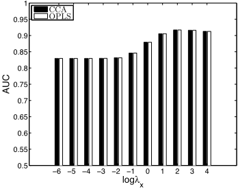
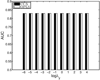
In this experiment, we use two multi-label data sets scene and yeast to verify the equivalence relationship between CCA and OPLS. The scene data set consists of 2407 samples of dimension 294, and it includes 6 labels. The yeast data set contains 2417 samples of 103-dimension and 14 labels. For both data sets, we randomly choose 700 samples for training. A linear SVM is applied for each label separately in the dimensionality-reduced space, and the mean area under the receiver operating characteristic curve, called AUC over all labels is reported.
The performance of CCA and OPLS on the scene data set as λx varies from 1e-6 to 1e4 is summarized in Figure 1. Note that in this experiment we only consider the regularization on X. It can be observed that under all values of λx, the performance of CCA and OPLS is identical. We also observe that the performance of CCA and OPLS can be improved by using an appropriate regularization parameter, which justifies the use of regularization on X.
We also investigate the performance of CCA and OPLS with different values of λy and the results are summarized in Figure 2. We can observe that the performance of both methods is identical in all cases, which is consistent with our theoretical analysis. In addition, we observe that the performance of CCA remains the same as λy varies, showing that the regularization on Y does not affect its performance.
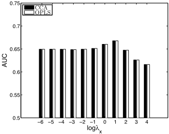
We perform a similar experiment on the yeast data set, and the results are summarized in Figures 3 and 4, from which similar conclusions can be obtained.
6 Conclusions and Future Work
In this paper we establish the equivalence relationship between CCA and OPLS. Our equivalence relationship elucidates the effect of regularization in CCA, and results in a significant reduction of the computational cost in CCA. We have conducted experiments on both synthetic and real-world data sets to validate the established equivalence relationship.
The presented study paves the way for a further analysis of other dimensionality reduction algorithms with similar structures. We plan to explore other variants of CCA using different definitions of the matrix H to capture the information from the other view. One possibility is to use the most important directions encoded in Y by considering its first k principal components only, resulting in robust CCA. We plan to examine the effectiveness of these CCA extensions in realworld applications involving multiple views.
Acknowledgement
This work was supported by NSF IIS-0612069, IIS-0812551, CCF-0811790, NIH R01-HG002516, and NGA HM1582-081-0016.
@inproceedings{ijcai2009p207,
  title     = {On the Equivalence between Canonical Correlation Analysis and Orthonormalized Partial Least Squares},
  author    = {Sun, Liang and Ji, Shuiwang and Yu, Shipeng and Ye, Jieping},
  booktitle = {Proceedings of the Twenty-First International Joint Conference on
               Artificial Intelligence, {IJCAI-09}},
  publisher = {International Joint Conferences on Artificial Intelligence},
  editor    = {Craig Boutilier},
  pages     = {1230--1234},
  year      = {2009},
  url       = {https://ijcai.org/proceedings/2009/207},
}
TY - CPAPER TI - On the Equivalence between Canonical Correlation Analysis and Orthonormalized Partial Least Squares AU - Sun, Liang AU - Ji, Shuiwang AU - Yu, Shipeng AU - Ye, Jieping T2 - Proceedings of the Twenty-First International Joint Conference on Artificial Intelligence, IJCAI-09 PB - International Joint Conferences on Artificial Intelligence PY - 2009 SP - 1230 EP - 1234 UR - https://ijcai.org/proceedings/2009/207 ER -Copied
Machine-readable versions of this paper, for tools and AI agents:





