
Semi-Supervised Classification on Evolutionary Data
Proceedings of the Twenty-First International Joint Conference on Artificial Intelligence. Pages 1083-1087.
© 2009 International Joint Conferences on Artificial Intelligence
Abstract
In this paper, we consider semi-supervised classification on evolutionary data, where the distribution of the data and the underlying concept that we aim to learn change over time due to short-term noises and long-term drifting, making a single aggregated classifier inapplicable for long-term classification. The drift is smooth if we take a localized view over the time dimension, which enables us to impose temporal smoothness assumption for the learning algorithm. We first discuss how to carry out such assumption using temporal regularizers defined in a structural way with respect to the Hilbert space, and then derive the online algorithm that efficiently finds the closed-form solution to the classification functions. Experimental results on real-world evolutionary mailing list data demonstrate that our algorithm outperforms classical semi-supervised learning algorithms in both algorithmic stability and classification accuracy.Yangqing Jia, Shuicheng Yan, Changshui Zhang
- [Belkin and Niyogi, 2005] Mikhail Belkin and Partha Niyogi. To- wards a theoretical foundation for laplacian-based manifold methods. In COLT, pages 486-500, 2005.
- [Belkin et al., 2006] M. Belkin, P. Niyogi, and V. Sindhwani. Man- ifold Regularization: A Geometric Framework for Learning from Labeled and Unlabeled Examples. JMLR, 7:2399-2434, 2006.
- [Chakrabarti et al., 2006] D. Chakrabarti, R. Kumar, and A. Tomkins. Evolutionary clustering. In KDD, pages 554-560, 2006.
- [Chi et al., 2007] Y. Chi, X. Song, D. Zhou, K. Hino, and B.L. Tseng. Evolutionary spectral clustering by incorporating tem- poral smoothness. In KDD, pages 153-162, 2007.
- [Dumais et al., 1998] S. Dumais, J. Platt, D. Heckerman, and M. Sahami. Inductive learning algorithms and representations for text categorization. In CIKM, pages 148-155, 1998.
- [Evgeniou et al., 2006] T. Evgeniou, C.A. Micchelli, and M. Pontil. Learning multiple tasks with kernel methods. JMLR, 6(1):615, 2006.
- [McCallum, 1996] A.K. McCallum. Bow: A toolkit for statistical language modeling, text retrieval, classification and clustering. http://www.cs.cmu.edu/˜mccallum/bow, 1996. Link
- [Ning et al., 2007] H. Ning, W. Xu, Y. Chi, Y. Gong, and T. Huang. Incremental spectral clustering with application to monitoring of evolving blog communities. In SDM, 2007.
- [Salton and McGill, 1986] G. Salton and M.J. McGill. Introduction to Modern Information Retrieval. McGraw-Hill, Inc., 1986.
- [Schölkopf and Smola, 2002] B. Schölkopf and A.J. Smola. Learn- ing with kernels. The MIT Press, 2002.
- [Zhou et al., 2003] D. Zhou, O. Bousquet, T.N. Lal, J. Weston, and B. Scholkopf. Learning with Local and Global Consistency. In NIPS, 2003.
- [Zhu et al., 2003] X. Zhu, Z. Ghahramani, and J. Lafferty. Semi- Supervised Learning Using Gaussian Fields and Harmonic Func- tions. In ICML, 2003.
- [Zhu, 2007] X. Zhu. Semi-Supervised Learning Literature Survey. Computer Science, University of Wisconsin-Madison, 2007.
References were extracted automatically from the PDF and may contain errors.
Full text extracted automatically from the PDF; figures, tables and equations may differ. The PDF is the version of record.
1 Introduction
Classification has been an important topic in the machine learning area for decades. In most of the classical applications, the data to be analyzed are considered as a whole set sampled from an unknown but fixed distribution. However, in many applications the distribution of the data and the underlying concept we aim to learn may change over time. Such changes often come from two factors: the short-term variation due to the noise, and the long-term drift of the underlying concept. A working example of the concept drift is that in online communities such as newsgroups, mailing lists and web news sites, the distribution of the posts on a certain topic may slowly change in the long term. For example, posts on the topic "Hi-Tech" may slowly drift from the space project in the 1960s to the emerging IT industry in the recent years due to the evolution of the society and public interest. Meanwhile, for most real-world applications, the drifting of the data distribution and the underlying concept is smooth over time, and does not take place sharply: a newsgroup tracing the development of AI may have been focusing on different research areas in the last decades, but is not likely to suddenly jump to focus on arts and literature. This creates what we call the evolutionary data and raises new challenges to traditional learning algorithms.
∗This work was supported in part by National Natural Science Foundation of China (Grant No. 60835002), and in part by AcRF Tier-1 Grant of R-263-000-464-112, Singapore. The work was performed when Yangqing Jia was a Research Engineer at the National University of Singapore.
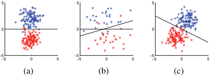
Similar to the nature of the evolutionary data, classification on evolutionary data learns a chain of evolving classifiers for different time periods. On the one hand, the classifiers are not identical to each other, and using historical classifiers makes little sense because the data distribution has changed during the time. Training a single classifier using all historic data also makes little sense, since the i.i.d. assumption of the classical classification algorithms does not hold in this case. On the other hand, the classification on the data should be smooth temporally, i.e., it should not deviate too much from the output of the classifier for the recent history, because the drifting of the data and the concept to learn does not change dramatically in most real-world applications. This indicates that historical classification information may help to determine the current classifier.
Figure 1 shows a toy example of the short-term fluctuation and long-term drifting. Assume that we are going to classify two Gaussians and know the classifier at a certain time that separates the two classes well as in (a). In the short-term scenario shown in (b), when there are only a few data with comparatively large noise, we may believe that the classification using the historical information (the dashed line) may be more reliable than the classification using the current data only (the dot dashed line), which reflects the idea of temporal smoothness. Also, in the long-term, when the positions of the two Gaussians evolve, the classification should also evolve to predict the new data accurately as shown in (c). Thus, evolutionary classification helps us both to suppress the short-term noise and to adapt well to the long-term concept drift.
In the unsupervised case, [Chakrabarti et al., 2006] first proposed evolutionary clustering to consider the evolving nature of the data, which can be considered as an unsupervised version of the problem we are considering. The basic thought is to minimizing the historical consistency along the time as well as the clustering quality for a certain time period. Based on such thought, [Chi et al., 2007] proposed evolutionary spectral clustering for general-purpose clustering problems. For real-world applications, [Ning et al., 2007] proposed to consider temporal evolving information for clustering to discover blog communities. However, to the best of our knowledge, there has been no prior work that considers semi-supervised classification for evolutionary data. In this paper we mainly focus on semi-supervised classification [Zhu et al., 2003], when only a small proportion of the data are labeled and the remaining are unlabeled. Specifically, we will first discuss how to utilize the temporal smoothness thought similar to the unsupervised case, and then propose a new semi-supervised learning algorithm for evolutionary data, which carries out temporal regularization in a structural way using the Hilbert space. Through real-world applications we demonstrate that our method offers better classification results than classical semi-supervised learning algorithms.
2 A Brief Review of SSL
First we give a brief view on the classical semi-supervised learning (SSL) problem. We will particularly focus on the idea of manifold regularization framework proposed by [Belkin et al., 2006] that is closely related to this paper.
In the semi-supervised learning problem, we are given a set of data points X = {x1, x2, · · · , xl, xl+1 · · · , xn}, where the first l data Xl = {xi}li=1 are labeled as Y = {yi}li=1 where yi represents the label of xi, and the remaining data Xu = {xi}ni=l+1 are unlabeled. Each datum xi ∈ X is sampled i.i.d. from a fixed but unknown distribution P(x) in the feature space Rd . The task of SSL is to learn the labels of the unknown data points (for transductive algorithms), or more ideally, the closed-form representation of the classification function f(x).
Belkin et al.proposed a general framework called manifold regularization [Belkin et al., 2006], which seeks an optimal classification function f by minimizing the following objective function:
where the first term L is a loss function defined on the labeled data points, such as the squared loss (yi - f(xi))2 for least-square problems, or the hinge loss function max[0, 1 - yif(xi)] for SVM. Two regularizers are adopted in this framework. The structural regularizer ‖f‖2K controls the function's complexity measure in an appropriately chosen Reproducing Kernel Hilbert Space (RKHS) HK of functions f : X → R, which is associated to a predefined Mercer kernel K: X ×X → R and has norm ‖ · ‖K. The spatial regularizer ‖f‖2I is a smoothness penalty term that reflects the intrinsic structure of the data distribution P(x). When the data lies on a low-dimensional manifold M(which generally holds if the dimensionality of the data is high), the term penalizes the function f along the manifold. γA and γI are two weight parameters set prior.
In most cases, we do not know the exact distribution P(x). [Belkin et al., 2006] showed that ‖f‖2I may be approximated using the labeled and unlabeled data as
where f = [f(x1), f(x2), · · · , f(xn)]⊤, and Wij is the edge weight in the data adjacency graph. L = D -W is the graph Laplacian matrix, where W is the weight matrix, and D : D(i, i) = ∑nj=1 Wij is a diagonal degree matrix. It has been proved in [Belkin and Niyogi, 2005] that by choosing Gaussian weights to construct the data adjacency graph as
where d(xi, xj) is the distance between xi and xj, the graph Laplacian converges to the Laplace-Beltrami operator ∇M or its weighted version on the manifold, which serves as a theoretically sound regularizer.
Several earlier semi-supervised learning algorithms, such as the Gaussian random fields and harmonic function method [Zhu et al., 2003] and the local and global consistency method [Zhou et al., 2003] can all be considered special cases under this general framework. We refer to [Zhu, 2007] for a complete survey on the semi-supervised algorithms.
3 SSL for Evolutionary Data: SSL-E
In this section, we introduce the semi-supervised learning algorithm for evolutionary data in detail. First, we discuss how to incorporate the temporal regularizer, and then develop both offline and online algorithms for this semi-supervised learning task.
3.1 Basic settings
When the classification task is carried out evolutionarily, we aim to learn a function F(t) : R ↦→ H, where H is a Hilbert space of classification functions f : Rd ↦→ R. Following the idea of SVM, we use a Reproducing Kernel Hilbert Space HK associated with a pre-defined kernel K. Specifically, F(t) = ft gives the classification function for each time t, and ft is then used to predict the label of the data generated from time t. For simplicity and real-world applications, we assume that the time t takes integer value from 1 to T. For example, posts of a mailing list from each month can be considered as data from one time step. Thus we are given a set of data sets X = {X1, X2, · · · , XT } that are from T consecutive time steps, which we call "frames", borrowing the idea from video processing. Each subset Xt = {x1,t, x2,t, · · · , xnt,t}1
1 For each data, the first subscript denotes the index in the dataset, and the second subscript denotes the index of the frame that the data belongs to.
contains nt data points that are generated from an unknown data distribution P(x; t) in the feature space Rd . Similar to the classical SSL problem, we assume that the first lt data {x1,t, · · · , xlt,t} are labeled as Yt = {yi}lt i=1 . In this way, the goal is to find T classification functions {F(t)}Tt=1 = {ft(x)}Tt=1 for all the frames that classifies the unlabeled data points and possible out-of-sample data. Similar to classical SSL algorithms, for the dataset Xt from each frame, a data adjacency graph can be constructed. We denote the weight matrix, the degree matrix and the graph Laplacian by Wt, Dt, and Lt respectively.
3.2 Evolutionary Smoothness Assumption
Recall the smoothness assumption in the general learning problems, which argues that two data points are likely to have similar labels if they are close to each other. We may extend it to the evolutionary data and make the following assumption when the label changes over time:
Evolutionary Smoothness Assumption: classification functions ft1 and ft2 are likely to be similar if the times t1 and t2 are close.
A direct approach to calculate the similarity is to use the integral of ‖∂F/∂t‖2 over time t. For a give time interval from 1 to ≤ T , the integral can be calculated as:
The smaller the integral is, the smoother the function is over the time. Consider the extreme case, when we force the integral to be zero, the classification functions will be identical with respect to the time t.
In the problem proposed in Section 3.1, we assume that the time takes discrete value from 1 to T. Thus, inspired by the work of [Evgeniou et al., 2006], we may use the backward difference to approximate the above integral as
where the norm ‖ · ‖K is carried out in the RKHS HK and compares the distance between the two classification functions ft and ft-1 in the RKHS.
3.3 Offline Learning Algorithms
Equation (5) serves as a temporal regularizer for the learning algorithm. We first propose an offline learning algorithm to show how to use the temporal regularization term. Taking into consideration the evolutionary smoothness assumption, an offline learning algorithm simultaneously learns the T classification functions by minimizing the following objective function:
where γA and γI are pre-defined weight parameters. Note that for t = 1, as there are no preceding frames, we carry out the temporal regularizer as ‖f1‖2K similar to the idea of support vector machines. It is not difficult to observe that the problem is convex if the loss function L is convex, thus the global optimal solution can be found.
3.4 The Representer Theorem
Although the convexity is guaranteed, it is still difficult to find the analytical form of {ft(·)}Tt=1 in the Hilbert Space. In the support vector machine and manifold regularization algorithms, the representer theorem [Sch¨olkopf and Smola, 2002; Belkin et al., 2006] enables us to convert the problem into finding a set of expansion coefficients. Actually, we can extend the representer theorem to the evolutionary case:
Theorem 3.1. (Representer Theorem) Assume that the regularizers ‖ft(·)‖2I (1 ≤ t ≤ T) are carried out empirically using the graph Laplacian as f ⊤ t Ltft where ft is the vector of function values {ft(xi,t)}, then the minimizer of (6) admits an expansion
given a predefined Mercer kernel K(·, ·).
In another word, each classification function can be expanded by the (∑Tt=1 nt) kernel functions {K(x, xi,k)}nt i=1 Tt=1 . The proof to the theorem is similar to the one in [Belkin et al., 2006] and is based on the orthogonality argument [Sch¨olkopf and Smola, 2002]. We provide the proof as follows:
Proof. (Theorem 3.1) In the RKHSHK, denote the subspace spanned by the kernel functions {K(·, xi,t)}nt i=1 Tt=1 by S. Thus, any function f ∈ HK can be decomposed as the sum of two orthogonal terms as f = f‖ + f⊥, where f‖ is the projection of f to the subspace S and f⊥ is the orthogonal complement. By definition, f‖ admits the expansion
According to the reproducing property of RKHS, for any data point xi,t (1 ≤ t ≤ T, 1 ≤ i ≤ nt), the function value is:
which turns out to be independent from the orthogonal part f⊥. Note that the second equal sign of the equation holds because 〈K(·, xi,t), f⊥〉 = 0 and the property of 〈K(·, x1),K(·, x2)〉 = K(x1, x2). Thus, the loss function and the empirical regularizers ‖ft(·)‖2I in (6) depend only on the value of the expansion coefficients {αi}nt i=1 Tt=1 and the predefined kernel K(·, ·).
For any two functions f and g in HK, they can be decomposed as the sum of the projection onto subspace S and the orthogonal complement as f = f‖ + f⊥ and g = g‖ + g⊥. Thus, we have
The second equal sign is because f‖-g‖ and f⊥-g⊥ are also orthogonal to each other. Consider the initial situation t = 1, the norm of function f1 in HK can naturally be written as
and non-zero orthogonal complement terms for any ft will increase the value of the loss function. Thus, the minimizer of (6) always admits the expansion as (7).
3.5 The Online Algorithm
In practice, especially for large-scale problems such as text mining, the offline learning algorithm may not work successfully as it requires to simultaneously learning the classification functions for all the frames. As the data accumulates, the learning problem scales up fast and renders the offline algorithm impractical. However, the offline algorithm and the representer theorem gives us a theoretical view of the problem and enables us to further consider more efficient online algorithms, which learn one classifier for the current frame with the historic information fixed.
Specifically, for each frame t (2 ≤ t ≤ T), the online learning algorithm finds the classification function ft(·) by minimizing the following objective function 2 :
where the classification function ft-1(·) is known.
It is not difficult to have the following corollary, which is the direct result of Theorem 3.1:
Corollary 3.1. Assume that the regularizers ‖ft(·)‖2I (1 ≤ t ≤ T ) are carried out empirically using the graph Laplacian as f ⊤ t Ltft, then for each frame t, the minimizer of (12) admits an expansion
given a predefined Mercer kernel K(·, ·).
The corollary represents the characteristics of a typical causal system: at time t, the classification function ft(·) is completely determined by the observations at and before t. However, notice that the problem of the offline algorithm still exists: as the data accumulates, the scale of the expansion subspace S that is constructed by the kernel functions {K(·, xi,k)}nk i=1 tk=1 may grow too large for learning. Thus, we manually impose a representer constraint to the optimization problem: for each frame f , we find the minimizer of (12) only in the subspace St = span{K(·, xi,t)|xi,t ∈ Xt} that is spanned by the kernel functions corresponding to the dataset Xt, i.e.,
2 Note that for t = 1, no historical information can be considered, so the algorithm deteriorates to the classical manifold regularization algorithm by replacing ‖ft(·) - ft-1(·)‖2K with ‖f1(·)‖2K.
Each subspace St is also a subspace of S. Note that the representer constraint actually narrows the solution space. If we assume that there are enough data in Xt, which is generally assumed in semi-supervised learning and satisfied in many real-world applications, empirically the subspace St is often enough to learn a good classification function. Thus, by adding the representer constraint we may find a good balance between computational speed and prediction accuracy.
3.6 Kernel Based Representation
In this subsection we give a kernel based representation for the online algorithm, and derive its closed-form solution. For each frame t, the solution to the online algorithm admits the expansion
Thus, denote by ft the nt × 1 column vector [ft(xi,t)], and denote by αt the nt ×1 column vector [αi,t], ft can be calculated by
where Kt is an nt × nt kernel matrix with its ij-th element be K(xi,t, xj,t). The regularizers in (12) can be respectively calculated by:
where Kt,t-1 is an nt × nt-1 kernel matrix with its ij-th element be K(xi,t, xj,t-1). Further, if we use the squared loss L(yi,t, xi,t, ft(·)) = (yi,t - ft(xi,t))2 , the objective function (12) can be written as (eliminating the constant terms)
where yt is the label vector [yi,t] (If the data point xi,t is unlabeled, yi,t may be set to any value, usually zero) and Ct is an nt ×nt diagonal matrix with its ii-th element be 1 if xi,t is labeled, and 0 otherwise. By setting ∂J (t) on /∂αt = 0, we have the optimum solution in the closed-form as
and
| Label | Date | Total Posts | Posts/Month |
|---|---|---|---|
| audiophiles | 2005.6 - 2008.9 | 35,666 | 892 |
| listening-l | 2003.7 - 2008.9 | 25,738 | 422 |
| sqlite-users | 2003.10 - 2008.9 | 32,655 | 544 |
| tutor-python | 2004.12 - 2008.9 | 26,314 | 572 |
| wine-devel | 2003.9 - 2008.9 | 41,302 | 677 |
3.7 The Influence of the Historic Data
In the online algorithm, the classification function at the current frame is only compared with the function in the previous frame. However, it is important to note that all the historic data actually influence the decision at the current frame. To see this, notice that the function ft(·) is determined by three terms: the supervised information, the data distribution at time t, and the function ft-1(·). In turn, ft-1(·) is determined by the data (including the supervised labels) at time t and the function ft-2(·). In this way all the historical information accumulates to determine the current prediction. We will provide an empirical example showing the accumulation of the historical information in Section 4.
4 Experiments
We test the effectiveness of our method on real-world evolutionary mailing list data, which reveals the evolutionary nature of data over a long time period in the text classification application. First we give a brief description about the data preprocessing. A web crawler was used to automatically retrieve posts of five online mailing lists from their mail archives, dated from September 2003 to September 2008. A total of 182,343 raw posts were collected. Mailing list identifying information such as the header of the posts and the signature lines of the corresponding list were removed before processing the text. Then, we applied rainbow [McCallum, 1996] to lex the data files, who removed 20,668 posts that are either non-text or contain too few words, and obtained a set of 161,675 posts for the learning task. Table 1 provides the general statistics of the datasets. Using the vocabulary produced by rainbow, we counted the number of occurrences of each word in each document and calculated the tf-idf value to form the feature vector for each document, which is further normalized to unit length. We refer to [Salton and McGill, 1986] for a detailed introduction about the tf-idf value and its physical interpretation. The corresponding mailing list of each post is used to label the post as the ground truth. Thus we have five classes of evolutionary data.
For the real-world dataset, classical semi-supervised learning incorporating all the current and historic data is not applicable, since the computation speed and required memory space both suffer from the large scale of the dataset. Thus, we applied three methods to analyze the data: the classical SSL algorithm that is performed separately on each frame, a naive evolutionary SSL that simply uses the data from the current frame and its preceding frame to learn the classifier, and online version of the algorithm SSL-E proposed in our paper. For all the methods, we used the linear kernel to define the RKHS, and used grid-search to find the optimal γI and γA for the best average performance over the frames on the experimental pair sql vs. win, which is then applied universally to other experimental pairs. The graph is constructed in a 10-nearest neighbor way, and the distance is calculated using the cosine similarity:
A smaller d(xi, xj) indicates that xi and xj are more similar to each other. Note that the linear kernel and cosine distance have been widely applied to applications in text classification such as [Dumais et al., 1998], and these settings are similar to the experimental settings that are used in [Belkin et al., 2006].
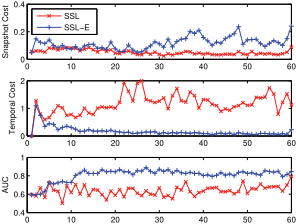
First we performed one-vs-one classification on the text data. For each experimental pair, we used the time period when both of them have posts and considered each month as a frame. 10 data points are randomly labeled for each frame (however, we ensure that there is at least one labeled post for each class) and the rest of them are unlabeled. The average value of the area under the ROC curve and the standard deviation over time are reported in Table 2. It is observed that the evolutionary algorithm clearly outperforms the standard semi-supervised learning algorithm that does not use temporal information, which justifies the effectiveness of the temporal regularizer. We further tested the performance of multiclass classification using data from all classes in the years from 2005 to 2008. For each frame, 10% of the posts are labeled, a little more than the one-vs-one case because considering multiple classes simultaneously adds to the difficulty of classification. The accuracy is reported in the last column of Table 2. Again, the evolutionary algorithm SSL-E performs much better than the classical SSL algorithm and naive evolutionary learning algorithm. To better show the inherent nature of the evolutionary algorithm, a comparison between SSL and SSL-E on the spatial cost and the temporal cost, which are the value of spatial regularizer (17) and temporal regularizer (5) respectively, are presented in Figure 2.
From the experimental results we may find the advantage of the evolutionary algorithm in two aspects. First, it helps to increase the classification accuracy in most cases. Second, from Figure 2 we can observe that the evolutionary algorithm can maintain a more stable performance than the classical SSL algorithm, which suggests that it is more robust against the noise in the data distribution and weak labeled information. Also, notice that the naive extension (SSL-naive) of the classical SSL using the current and precedent frames only achieves a limited increase in the performance. The reason is that for SSL-naive, the historical information only propagates from one frame to its direct follower but not any further. SSL-naive can of course use more frames to train the classifier, but again the large scale of the number of data points will render the solution impractical. Instead, SSL-E is able to accumulate all the historical information to assist the current frame, with only a minimal increase in the computation complexity.
| class | aud/lis | aud/sql | aud/tut | aud/win | lis/sql | lis/tut |
|---|---|---|---|---|---|---|
| SSL | 97.03 (4.42) | 96.12 (5.19) | 94.04 (7.05) | 93.14 (8.20) | 84.40 (9.02) | 81.50 (9.89) |
| SSL-naive | 97.77 (2.98) | 95.99 (6.39) | 95.47 (6.33) | 93.18 (10.28) | 86.30 (7.39) | 85.77 (8.38) |
| SSL-E | 98.98 (2.03) | 98.80 (2.97) | 97.95 (4.87) | 97.11 (6.89) | 92.74 (6.41) | 91.30 (6.65) |
| class | lis/win | sql/tut | sql/win | tut/win | Multi-class | |
| SSL | 78.41 (10.52) | 63.00 (5.26) | 64.42 (4.97) | 63.33 (4.40) | 77.49 (5.02) | |
| SSL-naive | 81.19 (9.86) | 64.52 (3.41) | 68.45 (4.16) | 65.57 (3.51) | 78.13 (4.89) | |
| SSL-E | 91.41 (6.89) | 76.87 (4.10) | 80.87 (8.16) | 78.56 (7.13) | 86.10 (3.21) | |
There are two interesting points that are worth mentioning. First, the first diagram in Figure 2 shows that SSL-E actually has larger spatial costs than SSL, but still has higher AUC values. This indicates that simply minimizing the spatial cost calculated empirically via graph Laplacian may not be optimal for classification, since the number of data points nt is limited and may be affected by the noise of the data. Second, from the third diagram we can observe that the accuracy of SSL-E increases from t = 1 to about 12 and becomes stable. This demonstrates the argument in Section 3.7: all the historical information (not only t - 1) accumulates and helps to determine the classification at time t. For our experiment, the performance stabilizes in about ten frames.
5 Conclusion
Learning the natural evolutionary information of the data is a new challenge in the machine learning research. On the one hand, the concept drifts during the time and makes a single aggregated classifier inaccurate for long-term prediction. On the other hand, the drifting is smooth if we take a localized view over the time dimension, which enables us to impose smoothness assumption for the learning task. In this paper, we mainly focus on the semi-supervised learning problem, and proposed a new algorithm for learning a series of evolving classification functions. The temporal regularizer is defined in a structural way using the difference between two classification functions in a given Reproducing Kernel Hilbert Space. We then derived the online algorithm that can efficiently find the closed-form solutions to the classification functions. Experimental results demonstrate that the proposed algorithm provides much better performances on realworld application in both stability and accuracy than classical semi-supervised learning algorithms.
@inproceedings{ijcai2009p183,
  title     = {Semi-Supervised Classification on Evolutionary Data},
  author    = {Jia, Yangqing and Yan, Shuicheng and Zhang, Changshui},
  booktitle = {Proceedings of the Twenty-First International Joint Conference on
               Artificial Intelligence, {IJCAI-09}},
  publisher = {International Joint Conferences on Artificial Intelligence},
  editor    = {Craig Boutilier},
  pages     = {1083--1087},
  year      = {2009},
  url       = {https://ijcai.org/proceedings/2009/183},
}
TY - CPAPER TI - Semi-Supervised Classification on Evolutionary Data AU - Jia, Yangqing AU - Yan, Shuicheng AU - Zhang, Changshui T2 - Proceedings of the Twenty-First International Joint Conference on Artificial Intelligence, IJCAI-09 PB - International Joint Conferences on Artificial Intelligence PY - 2009 SP - 1083 EP - 1087 UR - https://ijcai.org/proceedings/2009/183 ER -Copied
Machine-readable versions of this paper, for tools and AI agents:





