
Selecting Informative Universum Sample for Semi-Supervised Learning
Proceedings of the Twenty-First International Joint Conference on Artificial Intelligence. Pages 1016-1020.
© 2009 International Joint Conferences on Artificial Intelligence
Abstract
The Universum sample, which is defined as the sample that doesn't belong to any of the classes the learning task concerns, has been proved to be helpful in both supervised and semi-supervised settings. The former works treat the Universum samples equally. Our research found that not all the Universum samples are helpful, and we propose a method to pick the informative ones, i.e., in-between Universum samples. We also set up a new semi-supervised framework to incorporate the in-between Universum samples. Empirical experiments show that our method outperforms the former ones.Shuo Chen, Changshui Zhang
- [Asuncion and Newman, 2007] A. Asuncion and D.J. New- man. UCI machine learning repository, 2007.
- [Belkin et al., 2004] Mikhail Belkin, Irina Matveeva, and Partha Niyogi. Regularization and semi-supervised learn- ing on large graphs. In In COLT, pages 624-638. Springer, 2004.
- [Belkin et al., 2005] M. Belkin, P. Niyogi, and V. Sind- hwani. On manifold regularization. In Proceedings of the Tenth International Workshop on Artificial Intelligence and Statistics (AISTAT 2005), 2005.
- [Dai et al., 2008] Wenyuan Dai, Qiang Yang, Gui-Rong Xue, and Yong Yu. Self-taught clustering. In ICML '08: Proceedings of the 25th international conference on Machine learning, pages 200-207, New York, NY, USA, 2008. ACM.
- [Freeman, 1977] L.C. Freeman. A set of measures of cen- trality based on betweenness. Sociometry, 40(1):35-41, 1977.
- [Freeman, 1978] L.C. Freeman. 1979. Centrality in social networks: Conceptual clarification. Social Networks, 1(215-239), 1978.
- [Joachims, 1999] T. Joachims. Transductive Inference for Text Classification using Support Vector Machines. In MACHINE LEARNING-INTERNATIONAL WORKSHOP THEN CONFERENCE-, pages 200-209.
- MORGAN KAUFMANN PUBLISHERS, INC., 1999.
- [Joachims, 2003] T. Joachims. Transductive Learning via Spectral Graph Partitioning. In MACHINE LEARNING- INTERNATIONAL WORKSHOP THEN CONFERENCE-, volume 20, page 290, 2003.
- [Raina et al., 2007] Rajat Raina, Alexis Battle, Honglak Lee, Benjamin Packer, and Andrew Y. Ng. Self-taught learning: transfer learning from unlabeled data. In ICML '07: Pro- ceedings of the 24th international conference on Machine learning, pages 759-766, New York, NY, USA, 2007. ACM.
- [Sinz et al., 2008] F.H. Sinz, O. Chapelle, C. Santa Clara, A. Agarwal, and B. Scholkopf. An Analysis of Inference with the Universum. In Proceedings of the Twenty-First Annual Conference on Neural Information Processing Sys- tems (NIPS), pages 1-8, 2008.
- [Vapnik, 2006] V. Vapnik. Transductive inference and semi- supervised learning. Semi-Supervised Learning, pages 454-472, 2006.
- [Weston et al., 2006] Jason Weston, Ronan Collobert, Fabian Sinz, Léon Bottou, and Vladimir Vapnik. Infer- ence with the universum. In ICML '06: Proceedings of the 23rd international conference on Machine learning, pages 1009-1016, New York, NY, USA, 2006. ACM.
- [Zhang et al., 2008] D. Zhang, J. Wang, F. Wang, and C. Zhang. Semi-Supervised Classification with Univer- sum. In SIAM International Conference on Data Mining (SDM), 2008.
- [Zhou et al., 2004] D. Zhou, O. Bousquet, T.N. Lal, J. We- ston, and B. Scholkopf. Learning with Local and Global Consistency. In Advances in Neural Information Pro- cessing Systems 16: Proceedings of the 2003 Conference. Bradford Book, 2004.
- [Zhu et al., 2003] Xiaojin Zhu, Zoubin Ghahramani, and John Lafferty. Semi-supervised learning using gaussian fields and harmonic functions. In In ICML, pages 912- 919, 2003.
References were extracted automatically from the PDF and may contain errors.
Full text extracted automatically from the PDF; figures, tables and equations may differ. The PDF is the version of record.
1 Introduction
Semi-supervised learning (SSL) is an important topic, which uses both labeled and unlabeled samples. There is an abundance of literature about SSL, e.g. [Joachims, 1999; 2003; Belkin et al., 2004; Zhou et al., 2004; Zhu et al., 2003] and the references therein.
Graph based SSL is one of the important branches of the whole SSL literature, with the representative works such as [Belkin et al., 2004; Zhou et al., 2004; Zhu et al., 2003]. In these methods, a graph is built to describe the structure of the samples in space. Each sample is assigned a node, and the weight of the edge between two nodes corresponds the similarity of the two samples. Then a soft label function f is learnt based on certain consistency and continuity assumptions.
The concept of Universum sample has been introduced by [Vapnik, 2006]. It is defined as the sample that doesn't belong to any of the classes the learning task concerns. For example, in the task of classifying 5 against 8 in handwritten digits recognition, samples of other digits can be considered as Universum samples. The Universum sample is practically easy to get, even easier than the unlabeled sample, since there is so few requirement for it. Take, for instance, the text classification of political news against sports ones. All news from other categories, including economy, entertainment, science, etc. can play the role.
Several works have been done to use the Universum samples both in the supervised learning and SSL settings. In [Weston et al., 2006], the authors give a modified Support Vector Machine (SVM) framework, called U-SVM. [Sinz et al., 2008] gives an analysis of [Weston et al., 2006], suggesting that U-SVM seeks "a hyperplane which has its normal lying in the orthogonal complement of the space spanned by Universum examples" 1 . These two works both contain similar punishing terms in the formulation that require the decision values on Universum samples not far from zero. However the above two works are done under the supervised learning settings, and no unlabeled samples are used. [Zhang et al., 2008] is the first paper to address SSL with Universum samples. The authors suggest the following formulation
ˆ f and ˆy are only on the labeled and unlabeled samples. The Universum samples are taken as out-of-sample examples. In the third term of (1), the value f (x ∗ i ) is inducted from ˆ f . Therefore it can also drive the decision value at Universum samples to zero. However, no explanation is provided about why the Universum samples can be treated as out-of-sample examples in this paper. There may be one uncertainty: ˆ f in Reproducing Kernel Hilbert Space (RKHS) is learned from only the labeled and unlabeled samples. Using it to do the induction on Universum samples is based on the implicit assumption that the distribution of Unversum samples is the same with that of labeled and unlabeled samples. This may not be true sometimes.
All of the three works mentioned above are based on the same assumption: the decision values on the Universum samples should be close to zero. Equally this is to say that the decision boundary should be dragged towards where the Universum samples have been distributed. However, this assumption may sometimes be misleading. Consider the toy example in supervised learning setting (Fig.1(a)). The two classes could be linear separated. Thus SVM would give 100% classification accuracy on the training set (Fig.1(b)). When introducing some Universum samples between the two classes, as shown in Fig.1(c), U-SVM can also give the 100% accuracy. But when using another set of Universum samples (Fig.1(d)) and the same parameter setting as above, the performance of the trained classifier is severely damaged to the accuracy of only 55%. This is due to that the linear decision boundary is dragged towards the Universum samples on the left-hand side, while the optimized setting is to pass through just in between the two classes. This example gives us the idea that not all the Universum samples are useful and there should be some mechanism to filter out the damaging ones. Intuitively, we should keep the Universum samples which is posited in between different classes, since it gives the right direction to which the decision boundary should be dragged to.
1 This is the direct quotation from [Sinz et al., 2008]
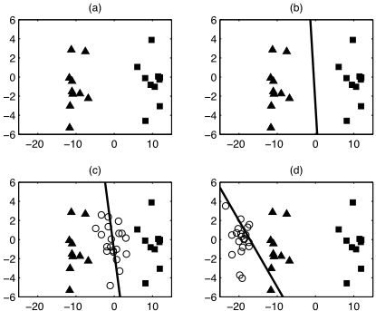
In this paper, we propose a method to select the in-between Universum samples (IBU) by using a modified version of betweenness centrality [Freeman, 1977; 1978]. An SSL framework is setup to incorporate the IBU, taking it as labeled sample rather that out-of-sample example. The experimental results on several datasets are promising.
The rest of the paper is organized as follows: In section 2, we give the notation and review the preliminaries for this paper. Our method of SSL using IBU is detailed in section 3, with experiments in section 4. We conclude our work and suggest future direction in section 5.
2 Notation and Preliminaries
In this paper, our methods only focuses on the binary classification case, while it can be extended to the multi-class scenario straightforwardly. Suppose we are given a dataset with three different parts. The first one is a labeled subset {(x l 1 , y1), (x l 2 , y2), . . . , (x l m , ym)} with m samples, where yi is corresponding label taking the value of ±1 for binary classification problems. The second one is an unlabeled subset {x u 1 , x u 2 , . . . , x u n } with n samples. And the third one is an Universum subset {x ∗ 1 , x ∗ 2 , . . . , x ∗ q }. x l i , x u j and x ∗ k are from the same input space χ where χ ∈ R d . We unify the three parts to {x1, x2, . . . , xm+n+q} so that
For supervised learning, only the labeled dataset is provided, while the unlabeled dataset is provided as complement in the SSL setting. The Universum dataset can serve both the supervised learning and SSL setting. We mainly focused on the SSL in this paper.
3 SSL Framework using IBU
In this section, we introduce our SSL framework using IBU. Firstly we give a brief introduction of the measure of centrality based on betweenness. Then we provide an algorithm to find the IBU using the defined measure of centrality. Finally, we set up the SSL framework to incorporate the IBU. The IBU is considered as labeled sample.
3.1 Betweenness of the Universum Samples
As mentioned in the introduction section, we hope to find the portion of the Universum samples that are in between samples from different classes. Thus a quantity to measure this betweenness is needed. We define it as
where σx l j ,x l k is the number of shortest paths on the graph from labeled sample x l j to labeled sample x l k . σx l j ,x l k (x ∗ i ) is the number of those paths that pass through the Universum sample x ∗ i . Intuitively, bU(x ∗ i ) gives a quantitative measure of to what extent Universum sample x ∗ i is in between any pairs of labeled samples from different classes. We can simplify the expression by letting σx l j ,x l k = 1, since the probability of existence of more than one shortest path between two vertices approaches zero when taking enough precision of the data into account. Thus the definition becomes
By using a manually set threshold t, we define IBU as
It is worth mentioning that our definition of betweenness is derived from the betweenness centrality in the graph theory and social network area ([Freeman, 1977; 1978]).
3.2 An Algorithm of Finding IBU
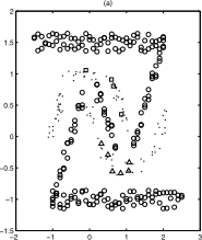
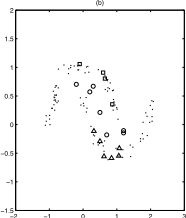
We give an algorithm to find IBU. The detail is listed in Table 1. The time complexity and space complexity are O((m + n + q) 3 ) and O((m + n + q) 2 ) respectively. We also give a simple demonstration on the well-known two-moon dataset with Universum samples added by us in Fig.2(a). We see that IBU do posit in between the two different classes. Also, the number of IBU is relatively small comparing to the whole Universum samples.
Input:
A dataset {x1, x2, . . . , xm+n+q}, with m labeled samples, n unlabeled samples and q Universum samples.
A label set {y1, y2, . . . , yn}for the labeled samples. A threshold t
Step 1:
Calculate the neighbor distance matrix G
where Nk(xi) is the set of the k-nearest neighbors of xi Step 2:
Initialize bU(x ∗ i ) = 0, 1 ≤ i ≤ q Step 3: for k = 1 : m + n + q for i, j = 1 : m+ n + q if Gik +Gk j < Gi j and m + n + 1 ≤ k ≤ m + n + q and yi nequal yj bU(x ∗ k-m-n ) = bU(x ∗ k-m-n ) + 1 end if Gi j = min(Gi j,Gik +Gk j) end for end for Output: The set of IBU UIB = {x ∗ i |bU(x ∗ i ) ≥ t}
-2
-1
0
1
2
3
-2
-1
0
1
2
3
Figure 2: The result of our finding IBU algorithm on the twomoon dataset with Universum samples. The distribution of provided samples are shown in (a). △ and □ stand for labeled samples from two classes respectively. ▪ is the unlabeled sample and © is the Universum sample. The result after our finding IBU algorithm is shown in (b), in which we use © to represent IBU found.
3.3 SSL Framework using IBU
As explained in the introduction part, treating the Universum samples as out-of-sample examples is unconvincing. We suggest to treat the IBU, which can be considered as the representative part of the Universum samples, as the labeled samples with label 0. So we reformulate the following optimization problem
|UIB| is the number of IBU. f is the predicted soft label, defined on labeled, unlabeled and IBU samples. y is the (m + n + |UIB|) × 1 given label vector, with its first m elements equal the label of labeled samples yi, while others 0. C is a diagonal weight matrix, with
C can be considered as the tradeoff between each parts of the samples. R is a regularization matrix. It can be the Laplacian or normalized Laplacian matrix on the labeled, unlabeled and IBU samples. The first term of (6) restricts f to be close to the given label on the labeled sample, and close to 0 on IBU. The second term is the regularization term that requires f does not change much on nearby samples. We denote our algorithm as Lap-IBU and NLap-IBU respectively. By setting the derivative of (6) to be 0, we obtain
The solution of this linear equation can be written in a pseudo-inverse form
This method avoids the mentioned problem of [Zhang et al., 2008] in the introduction part, because the labeled samples, unlabeled samples and IBU equally fit into the framework as a prior. This is to say that f is learned based on a mixture distribution of the three parts of samples. Also, as shown in the demonstration of last subsection, the number of IBU is small compared to that of the whole Universum samples. It won't affect the scale of the graph based SSL too much. One should notice that, this method can be considered as a special case of the framework in [Belkin et al., 2005], with the addition of IBU as labeled sample. The justification of the method can be found therein. Besides, we could do the induction on the out-of-sample examples when given a semi-definite kernel function k(· , ·) as
where K is the kernel matrix defined on labeled, unlabeled and IBU samples. k(x) is a (m + n + |UIB|) × 1 vector whose each element is the value of the kernel function applied on the out-of-sample example x and the provided labeled, unlabeled and IBU samples.
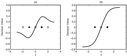
Moreover, we would like to show one possible good quality of our finding-IBU-strategy through an example in Fig. 3. Comparatively, the function learned from our method is less complex than that from the method of [Zhang et al., 2008]. Also in our method, the difference between the decision values of the two classes is greater. These mean that we could expect better generalization performances of our methods 2 . Intuitively, this is because we don't use the Universum samples that are not around the possible region of decision boundary. These samples would serve to "warp" the function towards zero on the periphery of the task-concerned data, and meanwhile affecting the decision value of the task-concerned data. Thus by discarding them, the learned function could be simplified, and the gap between two classed enlarged.
2 We assume that the to-be-predicted samples are task-concerned.
4 Experiments and Discussion
In this section, we conduct experiments on various datasets includingWine 3 , USPS 4 , MNIST 5 and Umist 6 to show the effectiveness of our methods. We compare our algorithm with four other ones, namely Lap-Universum, NLap-Universum, Lap-IBU* and NLap-IBU*. Lap-Universum and NLapUniversum are from [Zhang et al., 2008]. Lap-IBU* and NLap-IBU* use the same SSL framework as Lap-Universum and NLap-Universum, while incorporate IBU selected by our algorithm rather than the original Universum samples. We set Cl = 1 and k = kL = 15 (kL is the number of nearest neighbors in constructing the Laplacian or normalized Laplacian matrix). We also need to tune Cu, CU and the bandwidth σ in the RBF kernel.
4.1 Wine Dataset
The wine dataset is from the UCI machine learning repository ([Asuncion and Newman, 2007]). It contains 178 instances of wine from 3 different classes, each representing a wine cultivar. Each instance contains 13 attributes from chemical analysis. Our experiment is on the binary classification problem of class 1 (59 instances)and class 3 (48 instances), while using class 2 (71 instances) as Universum samples. For the class 1 and class 3 samples, we randomly pick part of them as the labeled samples. Others are treated as unlabeled samples. We vary the number of labeled samples and each setting is repeated 500 times. The average accuracy and the variance are listed in Table 2.
3 http://archive.ics.uci.edu/ml/datasets/Wine
4 http://cervisia.org/machine learning data.php
5 http://yann.lecun.com/exdb/mnist/
6 http://www.shef.ac.uk/eee/research/vie/research/face.html
| m | 5 | 10 | 15 | 20 |
|---|---|---|---|---|
| Lap-Universum | 83.26 ± 8.78 | 87.81 ± 3.43 | 88.90 ± 2.61 | 89.51 ± 2.54 |
| Lap-IBU | 85.70 ± 10.43 | 89.21 ± 3.89 | 90.24 ± 2.17 | 90.73 ± 1.93 |
| Lap-IBU* | 85.29 ± 10.34 | 88.42 ± 4.02 | 89.07 ± 2.83 | 89.45 ± 2.48 |
| NLap-Universum | 83.49 ± 9.99 | 87.47 ± 4.86 | 88.82 ± 3.24 | 89.73 ± 2.45 |
| NLap-IBU | 85.68 ± 11.36 | 88.97 ± 5.39 | 89.91 ± 2.86 | 90.81 ± 2.23 |
| NLap-IBU* | 85.20 ± 11.29 | 88.21 ± 5.51 | 88.99 ± 3.36 | 89.82 ± 2.56 |
4.2 USPS Dataset
The USPS dataset is a handwritten digit dataset scanned from envelopes. We used an abridged subset, with 200 samples for 2, 3, 5 and 8 respectively. Each sample is represented by a 256-dimensional vector extracted from the original 16 × 16 image. We test on the 5 vs 8 classification problem, with 2 and 3 treated as Universum samples. Different numbers of labeled samples corresponds different settings, which are repeated 50 times. The result is shown in Table 3.
| m | 5 | 10 | 15 | 20 |
|---|---|---|---|---|
| Lap-Universum | 92.41 ± 9.01 | 97.07 ± 1.95 | 97.49 ± 1.46 | 97.85 ± 1.19 |
| Lap-IBU | 93.18 ± 13.22 | 98.07 ± 1.57 | 98.48 ± 1.30 | 98.74 ± 0.85 |
| Lap-IBU* | 90.40 ± 13.89 | 96.90 ± 2.18 | 97.35 ± 1.88 | 97.68 ± 1.22 |
| NLap-Universum | 91.84 ± 8.67 | 93.26 ± 5.58 | 95.52 ± 3.00 | 95.60 ± 3.25 |
| NLap-IBU | 93.69 ± 11.52 | 97.29 ± 2.92 | 98.00 ± 1.28 | 98.36 ± 1.03 |
| NLap-IBU* | 87.80 ± 12.55 | 92.15 ± 5.75 | 95.13 ± 3.62 | 95.44 ± 3.34 |
4.3 MNISTDataset
MNIST Dataset is also a handwritten digit dataset with samples from 0 to 9. Each sample is a 16 × 16 image. For the 5 vs 8 classification problem, We select 100 5s, 100 8s and 1000 other digits uniformly distributed from the classes as the Universum samples. The numbers of randomly given labels are changed to form different settings, which is repeated 100 times. The result is listed in Table 4. We are also interested in what the IBU really are. So we pile the used IBU in the experiment up, and calculate the portion of each digit. They are listed in Table 5.
| m | 5 | 10 | 15 | 20 |
|---|---|---|---|---|
| Lap-Universum | 73.29 ± 10.92 | 80.44 ± 7.29 | 84.31 ± 4.94 | 86.47 ± 4.44 |
| Lap-IBU | 75.01 ± 11.03 | 83.27 ± 6.95 | 87.16 ± 4.53 | 89.18 ± 4.00 |
| Lap-IBU* | 74.24 ± 10.98 | 81.34 ± 7.28 | 84.48 ± 4.97 | 86.64 ± 4.65 |
| NLap-Universum | 83.49 ± 9.99 | 87.47 ± 4.86 | 88.82 ± 3.24 | 89.73 ± 2.45 |
| NLap-IBU | 85.68 ± 11.36 | 88.97 ± 5.39 | 89.91 ± 2.86 | 90.81 ± 2.23 |
| NLap-IBU* | 85.20 ± 11.29 | 88.21 ± 5.51 | 88.99 ± 3.36 | 89.82 ± 2.56 |
| Label | 0 | 1 | 2 | 3 | 4 | 6 | 7 | 9 |
| Percentage | 7.50 | 23.46 | 4.23 | 24.43 | 4.84 | 18.38 | 1.33 | 15.84 |
4.4 Umist Dataset
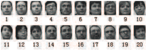
Umist dataset is a collection of 575 28 × 23 images of faces from 20 people, among which there are 4 female and 16 male (Fig. 4). We test on the classification of person 9 and person 20, two females, using samples of other 18 people as Universum samples. The accuracy against the number of labeled samples m is shown in Table 6, where each setting is repeated 100 times. We follow the setup of the experiment on MNIST and inspect the constituent of the IBU collection. It only contains two persons, 8.33% of person 6 and 91.67% of person 7.
| m | 5 | 10 | 15 | 20 |
|---|---|---|---|---|
| Lap-Universum | 91.56 ± 9.76 | 95.87 ± 4.50 | 96.69 ± 4.68 | 97.74 ± 2.65 |
| Lap-IBU | 94.24 ± 9.52 | 98.37 ± 2.58 | 99.09 ± 2.53 | 99.39 ± 1.77 |
| Lap-IBU* | 93.72 ± 9.60 | 98.13 ± 2.77 | 98.70 ± 2.85 | 99.11 ± 1.83 |
| NLap-Universum | 93.85 ± 0.55 | 97.02 ± 0.20 | 99.20 ± 0.004 | 99.50 ± 0.03 |
| NLap-IBU | 96.93 ± 0.48 | 99.07 ± 0.05 | 99.83 ± 0.01 | 99.91 ± 0.01 |
| NLap-IBU* | 98.43 ± 0.42 | 99.81 ± 0.01 | 100.00 ± 0.00 | 100.00 ± 0.00 |
4.5 Discussion
From the result of our experiments, we can tell that our methods based on IBU outperforms the former ones using the whole Universum dataset equally. The accuracy of using both Laplacian and normalized Laplacian favors ours algorithm. Besides, while both incorporating IBU, the methods of our SSL framework is better than that of former SSL framework in most cases. The only exception is that on the Umist dataset with normalized Laplacian matrix. These results show that: i).Using IBU is the main reason for the improvement of accuracy; ii). Our SSL framework is better than the former one under most of the circumstances. Moreover, the experiments give an intuitive demonstration of what IBU is like. In Table 5, digit 3 takes the greatest part of the IBU. This is mainly because 3 looks like both 5 and 8, justifying its high betweenness. In other word, 3 is the most useful Universum of classifying 5 and 8. This result coincides with [Sinz et al., 2008]. Digits 1, 6 and 9 as Universum also contribute to the problem greatly. Similarly in the experiment on Umist dataset, person 7 is important in the person 9 vs 20 classification task because it is also female.
We would like to give an explanation about how IBU works based on the experiment results. As shown above, IBU resembles both of the samples from two classes. Equally that is to say IBU can be taken as a "transition phase" of the two classes. Thus it can be helpful in following ways: Where the IBU lies represents a region that intercepts the changing trace from one class to the other class. Also it is a region that belongs to neither class. These characteristic is compatible with that of decision boundary and we use it as a guide to find it.
5 Conclusion and Future Work
In this paper, we research on the use of Universum sample, which is defined to be the sample that belongs to neither of the concerned classes. We suggest that not all the Universum samples should be treated equally, which is not realized in the existing works. An algorithm and a framework are proposed to pick the useful portion of Universum samples, defined as IBU, and incorporate them for the SSL setting. The results of experiments show that our methods is advantageous in predicting accuracy against the former ones. The experiments also give a demonstration of what IBU is - the "transition phase" between different classes.
The learning with Universum is related with some other fields of machine learning. [Zhang et al., 2008] refers the relations with multi-class and ordinal regression problem. A new proposed branch - self-taught learning, is also connected with the problem of learning with Universum ([Raina et al., 2007; Dai et al., 2008]). In the self-taught setting, one is provided with two parts of samples. One part contains the samples that belong to the classes the problem concerns. It could be labeled for the supervised learning or unlabeled for the clustering setting. The other part contains a great amount of randomly picked samples with no labels, which could belong to the classes the problem concerns or not. In our term, the second part includes unlabeled samples and Universum samples, with no indication of which is which. Self-taught methods use the second part of samples to assist the task defined originally on the first part. Since we cannot distinguish the unlabeled samples and the Universum samples, it cannot be adapted to learning with Universum framework directly.
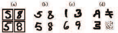
Besides, as a more general framework, there are four kinds of samples we may encounter in a learning problem. We list them in a descending order of importance: labeled sample, unlabeled sample, "unrelated" sample and "out-of-domain" sample. The "unrelated" sample is the sample that shares the same domain with the labeled and unlabeled sample, whereas does not belong to any of the concerned classes. The "out-of-domain" sample is the sample other than the defined three kinds. The mixture of "unrelated" sample and "out-ofdomain" sample is the Universum sample. We give an illustration of each kinds of samples in the 5 vs 8 classification problem (Fig. 5).
The existing learning problems using different combination of the four kinds of samples are listed in Table 7. Obviously, the four kinds of samples carry different amount of a priori. One possible future work is to set up a general framework to incorporate all the combination of the four kinds of samples and their mixtures.
| Provided Samples | Learning Problem |
|---|---|
| 1.Labeled Samples | Supervised Learning |
| 1.Unlabeled Samples | Clustering |
| 1.Labeled Samples 2.Unla- beled Samples | Semi-Supervised Learning |
| 1.Labeled Samples 2.Mixture of "Unrelated" Samples and "Out-of-domain" Samples | Supervised Learning with Universum |
| 1.Labeled Samples 2.Unla- beled Samples 3.Mixture of "Unrelated" Samples and "Out-of-domain" Samples | Semi-Supervised Learning with Universum |
| 1.Labeled Samples 2.Mixture of Unlabeled Samples, "Unre- lated" Samples and "Out-of- domain" Samples | Self-Taught Learning |
| 1.Unlabeled Samples 2.Mix- ture of Unlabeled Samples, "Unrelated" Samples and "Out-of-domain" Samples | Self-Taught Clustering |
Acknowledgments
This work is supported by the National Natural Science Foundation of China (Grant No.60835002 and 60721003). We would like to thank Yangqiu Song, Dan Zhang, Jianwen Zhang, Zheng Wang, Chenping Hou, Feiping Nie and Kun Gai for their help. We also appreciate the valuable comments by the anonymous reviewers.
@inproceedings{ijcai2009p172,
  title     = {Selecting Informative Universum Sample for Semi-Supervised Learning},
  author    = {Chen, Shuo and Zhang, Changshui},
  booktitle = {Proceedings of the Twenty-First International Joint Conference on
               Artificial Intelligence, {IJCAI-09}},
  publisher = {International Joint Conferences on Artificial Intelligence},
  editor    = {Craig Boutilier},
  pages     = {1016--1020},
  year      = {2009},
  url       = {https://ijcai.org/proceedings/2009/172},
}
TY - CPAPER TI - Selecting Informative Universum Sample for Semi-Supervised Learning AU - Chen, Shuo AU - Zhang, Changshui T2 - Proceedings of the Twenty-First International Joint Conference on Artificial Intelligence, IJCAI-09 PB - International Joint Conferences on Artificial Intelligence PY - 2009 SP - 1016 EP - 1020 UR - https://ijcai.org/proceedings/2009/172 ER -Copied
Machine-readable versions of this paper, for tools and AI agents:





