Self-Managing Associative Memory for Dynamic Acquisition of Expertise in High-Level Domains

1 Introduction

Associative memory is a frequently useful component for intelligent systems, allowing efficient lookup of relevant past experiences from a new situation. The requirements for an associative memory are very different, however, depending on whether it is being applied to store low-level or high-level models. In low-level applications, such as phoneme recognition or extraction of primitive visual features, the distribution of models, once learned, can be used quite generically and may be expected to shift little over time. In high-level applications, however, such as episodic memory or analogical reasoning, the models are likely to vary greatly from domain to domain.

Imagine a robotic clerk deployed in a hardware store. In order to help customers with questions, it will need to have expertise in a number of extremely different high-level domains, such as inventorymanagement, plumbing, and carpentry. Each such domain implies a collection of domain-specific models in its associative memory. If the hardware store begins carrying garden supplies, then the robotic clerk will need to be able to acquire domain expertise in gardening as well, and reallocate its associative memory to make room for a collection of models for the gardening domain.

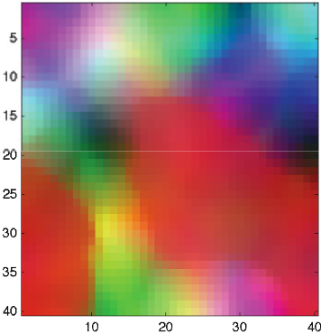
Self-organizing maps are an attractive option for implementing associative memory: they are fast, easily parallelized, and digest a stream of incoming data into a topographically organized collection of models where more frequent classes of data are represented by higher-resolution collections of models (e.g. Figure 1). Previously, however, the study of self-organizing maps has focused mainly on "configure once" maps that do not undergo significant shifts in structure once their initial configuration is complete.

In the absence of a general theory of SOMs, we use a mixture of analysis and empirical studies to characterize the behavior of SOMs for shifting input data from high-level domains, finding that new high-resolution collections of models develop quickly. High-resolution areas of the SOM decay rapidly unless actively refreshed, but in a large SOM, the ratio between growth rate and decay rate may be high enough to support both fast learning and long-termmemory.

2 RelatedWork

Self-organizing maps, also known as Kohonen networks, were first introduced in [Kohonen, 1982], and have been considered as a model of associative memory from the beginning [Kohonen, 1984]. Although their behavior has been analyzed precisely for the 1-dimensional case[Erwin et al., 1992], no general theory has yet been established to describe the behavior of SOMs with two or more dimensions. For a thorough review of the subject, see [Kohonen, 2001].

Self-organizing maps were originally proposed as a neural network modelling possible brain structure. Many other implementations of associative memory, such as Hopfield networks[Hopfield, 1982], are also neural network models and often suffer problems of poor retention or low storage capacity. Many other associative memories are essentially databases (the simplest being hash-tables and LISP alists), and simple versions have often been implemented in hardware under the name "content addressable memory" (e.g. [Chisvin and Duckworth, 1989]).

Although SOMs have been applied to high-level domains, they have generally been considered in terms of a single domain and the focus of research has generally been on how to map high-level structures effectively into vectors of numeric features (e.g [Fornells et al., 2006]). A notable exception is Tardiff 's work on Self-Organizing Event Maps[Tardiff, 2004], which uses symbolic models and blends by finding covers in an ontology of symbol classes.

While a few others (e.g. [Fornells and Golobardes, 2007; Hattori et al., 2001]) have begun to consider incremental adjustment of SOMs in response to changing data, these these have all worked with limited use of a small SOM and provided no evidence of the generalizability of SOMs for highlevel associative memory.

3 Model

Our investigation of self-organizing maps for high-level associative memory uses the standard self-organizing map definition, slightly generalized and with a minor variation to support distributions that change over time. We then model the distribution of high-level domain data as a collection of highmass 1 probability spikes against a background of noise.

3.1 Self-Organizing Maps

A self-organizing map consists of a collection of models Mi, distributed in some space-filling geometric arrangement, and functions for model lookup and adjustment. In this work, we consider two-dimensional SOMs where the models are arranged in a grid in Euclidean space, but expect that our results can be extended to higher dimensions and less restrictive topologies. 2

1 A probability mass function gives the probability that a discrete random variable is equal to some value. We use this terminology to emphasize that spikes are "nearly discrete."

The models are initialized randomly, then adjusted by a sequence of input data, ξ0, ξ1, . . . , added one by one to the SOM. The tth datum, ξt is looked up in the map by applying a match quality function Q(Mi, ξt), and selecting the bestmatching model b. 3 The datum is then blended into every model using a blending function

to produce an adjusted model M ′ i , where w is a weighting based on the geometric distance d(b, i) between model i and the best model b. The weight is in the range [0, 1], where 0 means the model is not changed at all and 1 means the datum entirely replaces the existing models. Weight decreases monotonically from a maximum at model b, possibly reaching zero at some finite distance.

The models can contain any sort of data, so long as they support the blend function B and match quality function Q. This is a generalization on the standard formulation, which uses k-dimensional vectors as models. The other difference from the standard model is that the standard model includes time in the weight function and later samples are given less weight. To allow the SOM to quickly reflect changes in the underlying distribution, we omit this effect from our model, though this does make the initial configuration of the SOM much slower and less globally coherent. 4

3.2 High-Level Data Distribution

The most salient characteristic of high-level domain data that concerns us is its sparse, clustered distribution. Memory fragments about plumbing, for example, may resemble one another vastly more than they resemble fragments about inventory management or gardening. Within plumbing, fragments about toilets may resemble one another vastly more than they resemble fragments about sinks or bathtubs. The precise relationships depend on the particulars of representation, of course, but some empirical justification for this assertion may also be found in the large gaps between basic categories in hierarchical clustering of human similarity judgements (e.g. [Tenenbaum and Xu, 2007]).

2 The particular choice of two dimensions comes from a combination of biological inspiration, since it has often been suggested that sections of the mammalian cortex may act as SOMs (e.g. [Kenet et al., 2003]), and ease of visualization.

3 We may assume that if ties occur, they are broken arbitrarily.

4 A hybrid model could likely have the best of both worlds, but is not of interest for this investigation, where we are primarily concerned with acquisition of expertise in new domains.

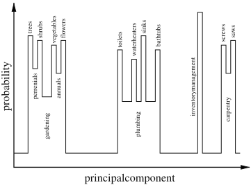
In order to characterize the behavior of an SOM learning about high-level domains, we thus use a simplified model of a distribution of high-probability spikes against an even background of noise. For a sample drawn from a distribution of k domains, there is a likelihood pi of the sample being drawn from the ith domain, and a likelihood 1 - ∑i<k pi of the sample being drawn uniformly from the space of all possible models, representing the vast number of possible domains that the system might cross paths with, but not often enough to develop expertise. For example, the experiences of the hardware clerk robot might be modelled using four spikes of varying masses for gardening, plumbing, carpentry, and inventory management (Figure 2), against a background level of noise for random experiences. The structuring of a domain into sub-domains may then be modelled by using a similar spiky distribution to draw samples from a domain. For example, the plumbing domain might have four spikes-toilets, sinks, bath-tubs, and water heaters-against a background of noise representing all other plumbing information.

Samples are drawn independently from this distributionstrong correlations can be modelled by changes in the distribution. For example, a training course on gardening would be a temporary shift to a distribution with high probability mass in the gardening spike and none on plumbing, carpentry, and inventory management.

4 Analysis and Empirical Characterization

Since there is not yet a general theory of self-organizing maps, we evaluate their suitability for high-level associative memory through a mixture of limit case analysis and empirical characterization.

4.1 Domain-Specific Regions and Noise Regions

Assume a large SOM where the models are arranged homogeneously in a low aspect-ratio area, and that input data is drawn from a k spike distribution as given in Section 3.2. Assuming that the background noise is non-negligible, we may expect the SOM's models to generally be arranged into k regions of domain-specific models, each separated from all of the others by regions of background noise models. The reason for such separation is simple: if two domain-specific regions happen to be in contact, then because the domains are sparse on the space of possible models, as samples are added they will results in blending along their border that creates continuum of intermediate models matched by noise and not by either domain.

We may thus begin our analysis by thinking of the boundary between a domain-specific region and a noise region. In the noise region, there is much more difference between neighboring models than in the domain-specific region. When domain-specific samples match models near the boundary, they make the models in the edge of the noise region more like the domain-specific models, incrementally moving the boundary outward and expanding the domainspecific region. Conversely, when noise samples match near the boundary, the boundary moves inward and the domainspecific region shrinks.

The size of a domain-specific region is thus regulated by the relative likelihood of domain samples and noise samples arriving at its boundary. Its shape will tend toward circular, since any deviation from circular increases the local nearboundary area of the opposing region, increasing the probability of incremental shifts that decrease the deviation.

4.2 Initial Growth of a Representation

Even though noise potentially draws samples from every domain, the narrowness of any particular domain means that when an SOM begins to develop expertise in a high-level domain, there will be few or no domain-specific models already existing. Initially, then, a large SOM will have vastly more noise models than models in the domain-specific region, and to a first approximation, all boundary motion will come from domain-specific models pushing the boundary outwards, since the area near the boundary is a small fraction of the total area of the noise region.

Assuming circularity, the area near the boundary grows as O(√n) (by area/circumference ratio), where n is the number of models in the domain-specific region, and each new example may be expected to have approximately the same effect. The likelihood of a sample being in the boundary is thus O(1/√n), and we can find the expected area after t samples by solving the differential equation dn dt = k/√n, where k is an unknown constant, yielding an expected growth rate of O(t2/3 ).

For an empirical verification of this result, we use a square SOM with side s = 100, containing 10,000 total models. The models are RGB colors-this simple and intuitive space will allow us to visualize models easily, while still having a dimensionality higher than the SOM itself, and should thus give us valid results so long as we use a spike-and-noise distribution. In this case, we choose a distribution with a single spike of mass m0 = 0.8, where samples are drawn uniformly from a cube of side ϵ = 0.05 centered on the red color (0.9, 0.1, 0.1), while noise is drawn uniformly from the entire space. Note that at 1/8000th of the area of the color space, noise that happens to land in the spike will have a minimal effect. Finally, the blend will be linear, with weight

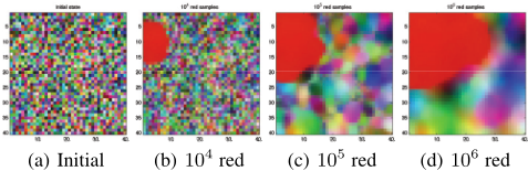
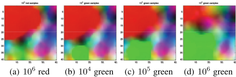
where the constants are set to α = 0.1 and r = 2, respectively, and the distance between grid neighbors is 1. We will use these same values for s, m0, ϵ, α, and r hereafter, except where otherwise noted. Figure 3 shows an example of how such an SOM develops (though with side 40 rather than 100).

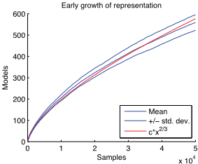
Figure 4 shows the result of 40 runs of 50,000 samples, counting domain-specific models every 100 samples and judging a model to be describing the red domain if it is within ϵ of the center of the cube (twice the range of generation). As predicted, the number of models n devoted to the red domain grows proportional to t3/2 , although by 50,000 samples the domain-specific models are approximately 5% of the SOM, and the mean is bending downward as the negligible noise assumption begins to fail.

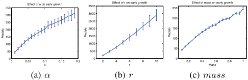
The blend parameters α and r and the domain mass m0 were not involved at all in our analysis, and thus should act linearly on the rate of growth (at least for small values of α and r). Experiment confirms this: Figure 5(a) shows the number of domain-specific models after 10,000 samples for α ranging from 0.01 to 0.19 in steps of 0.01, with 40 runs per value, Figure 5(b) shows the same for r ranging from 2 to 10, and Figure 5(c) shows the same for m0 ranging from 0.1 to to 1.0 in steps of 0.05.

4.3 Stable State

If the SOM started with only domain-specific models, then noise regions would appear and grow according to the same logic as for the growth of a domain-specific region. As such, we may expect the SOM to eventually reach a stable state in which the number of models devoted to a domain is determined only by the probability masses of the various domains and background noise.

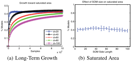
Since the equilibrium results from a balance of forces, it is natural to predict that the area will converge toward this final state at an exponentially decreasing rate. Figure 6 shows that these predictions hold. Figure 6(a) shows that the fraction of models representing the red domain at various side lengths converges exponentially to a stable value, counting domainspecific models every 100,000 samples for 10 million samples and running 40 times with each side length. Figure 6(b) shows that the fraction of models representing a spike after 10 million samples is nearly constant with respect to side length ranging from 5 to 100 in steps of 5 (25 to 10,000 models) and running 10 times with each side length. The slightly lower values of low side-length SOMs may be due to quantization of the low diameter and number of models, while the slightly lower values of high side-length SOMs are likely due to their continued slow convergence.

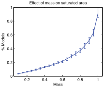
Mass, however, appears to have an unexpected effect on the final fraction of domain-specific models. Figure 7 shows the fraction of domain-specific models after 1 million samples in a 40 × 40 SOM with mass m0 varying from 0.05 to 1.0 in steps of 0.05 and running 40 trials per mass. Surprisingly, the relationship is clearly quadratic rather than linear, and the reason for this effect is not immediately obvious.

4.4 Changing Domain Expertise

With a first-approximation model of how domain-specific expertise can develop, we can now turn to the question of what happens when the set of high-level domains changes. This might be either a long-term shift or a short-term shift. For SOMs to be a good high-level associative memory, the system must be able to acquire new expertise quickly and have existing expertise decay slowly.

To characterize SOM behavior, we consider three basic cases of distribution change:

• A new domain joins existing domains (e.g. adding garden supplies to the hardware store)
• A shift from one domain to another (e.g. taking a training course on gardening)
• All domains are allowed to decay (e.g. abnormal tasks while the store moves to a new location)

Figure 8 shows a typical example of SOM evolution following a "shift"-case distribution change.

What can we predict about these cases? First, if adding a new domain reduces the overall noise level, then the nonlinearity of the mass curve in Figure 7 means that any preexisting domains can actually be expected to rapidly expand the number of models that represent them. Likewise, if a high-level domain is not included in the distribution, then the area representing it will be continuously encroached upon by background noise-though slower and slower as the area of the domain-specific region drops, and with it the size of the near-boundary area. Finally, we can expect that the initial growth rate for new high-level domains will be t2/3 as before-and with a higher constant due to the mass nonlinearity if there are other domains in the distribution.

The actual number of samples it takes to acquire expertise in a new domain is of fairly low importance. Depending on how the memory is being used, a complex chunk of continuous experience could be interpreted as anything from single item to be stored or a collection of thousands of different related parsings (different time boundaries, different details included and omitted, etc.). What is important is the relative speeds of growth and decay: if expertise in a domain is to be retained when it is not actively being used, then the rate at which unused expertise decays must be much slower than the rate at which new expertise in a domain is gained.

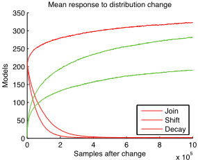
To examine these relative rates, we turn once again to empirical characterization, adding a green domain centered on (0.1, 0.9, 0.1), with the same ϵ as the red domain and its own independent mass m1. First, the SOM is trained on 1 million samples from a distribution with the red spike at m0 = 0.4, then the distribution is changed and training continues. In the "join" condition, m0 remains at 0.4 and m1 is set positive, adding a green spike; in the "shift" condition, m1 becomes positive and m0 is set to zero, and in the "decay" condition, both m0 and m1 are zero.

The number of models representing each domain changes with time as predicted following each of the three cases of distribution change. Figure 9 shows the mean result of 40 runs of 1 million samples for each of the three cases, with side length s = 40, masses m0 = m1 = 0.4, and counting domain-specific models every 1000 samples. As predicted, the red domain rises, at first rapidly, in the "join" case and drops more rapidly in the "decay" case where there is 100% background noise than the "shift" case there is 60% noise. Likewise, the green domain rises more rapidly and toward a higher final level in the "join" case than the "shift" case-and in both cases its initial growth is pleasingly fast.

To investigate whether the growth/decay ratio is reasonable, we consider two statistics: the length of time for the number of models representing the red domain to halve, and the time it takes for the green domain to reach 100 models. Figure 10 shows the two statistics for side length s ranging from 5 to 100 in steps of 5, with 40 runs for each length, and for a green domain mass ranging from 0.1 to 0.6 in steps of 0.05, with 40 runs for each mass. Decay time rises approximately quadratically with side length, indicating that the red domain is losing exterior models at a constant rate from the same approximate converged percentage, and also rises quadratically with increasing m1, which is unsurprising given the mass non-linearity. Growth behaves as before, so long as it is far from saturation.

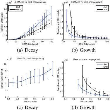
In the best conditions tested, growth is approximately one order of magnitude faster than decay. Since the time to decay will continue to rise as SOM side length rises, we may expect that increasing the side-length of the map tenfold will allow an SOM that can attain novice knowledge of a new high-level domain in a few days yet still retain some expertise after a decade of neglecting a well-studied domain.

Expertise that grows proportional to t2/3 and decays linearly is still worthy of concern. Part of the reason that this can happen is that updates of the SOM focus only on expanding a region that is being added to. A neglected region is inert, and can only be eaten away at by neighboring regions-and this also means that when there are many highlevel domains in the map, a neglected domain can be quickly destroyed entirely by a growing neighbor! An adjusted model in which models attempted to shift away from a growing region could address this, yet not require any more time when implemented in parallel. Instead of neglected domains being chewed away at their borders, they would instead slowly move away, compressing as they moved.

5 Contributions

Analysis and empirical characterization show that selforganizing maps can be used to implement associative memory for high-level data, even when the system must learn about new domains dynamically. Although neglected domains decay rapidly, a large SOM may have enough models to still support both fast learning of new domains and longterm retention of expertise.

This work is only a first-approximation characterization, enough to determine that it is worth pursuing SOM-based high-level associative memory. Following this, there are two main avenues for advancing this research. On the one hand, the current analysis and characterization can be extendedkey points to be addressed are the non-linearity of the mass relation, prediction of constants as well as scaling, hierarchical distributions (for domains that are, themselves structured), and SOMs with non-regular grids (whether from design or from accumulation of failures over time). On the other hand, as noted in the last section, the SOM algorithmmight be varied to shift data away from growing regions-expensive on a serial computer but cheap on parallel hardware.